For all those amateur Machine Learning and Deep Learning enthusiasts out there, Linear Regression is just the right way to kick start your journey. If you are new to Machine Learning with some background in PyTorch, then buckle up because you have just ended up at the right spot. In case you are not, don’t worry, checkout my previous article to pick up some fundamentals of PyTorch and then you are all good to go.

F或所有这些业余的机器学习和深度学习爱好者在那里，线性回归仅仅是开始踢你的旅程，以正确的方式。 如果您是刚接触PyTorch的机器学习的新手，那么请紧扣一下，因为您刚刚来到了正确的位置。 如果您不是，请不要担心，请查看我以前的文章以了解PyTorch的一些基础知识，然后一切都很好。

那么什么是线性回归？ (So what is Linear Regression ?)

Linear Regression is a linear model that predicts the output, given a set of input variables, assuming that there is a linear relationship between the input variables and the single output variable.

线性回归是在给定一组输入变量的情况下预测输出的线性模型，假设输入变量和单个输出变量之间存在线性关系。

For instance let’s just consider the simple linear equation y = w*x + b. Here y is the output and x is the input variable. “w” and “b” forms the slope and y intercept of the equation respectively. So we will refer to “w” and “b” as the parameters of the equation because once you get to know these values, you can easily predict the output for a given value of x.

例如，让我们考虑简单的线性方程y = w * x + b。 此处y是输出，x是输入变量。 “ w”和“ b”分别形成方程的斜率和y截距。 因此，我们将“ w”和“ b”称为方程式的参数，因为一旦了解了这些值，就可以轻松预测给定x值的输出。

Now let’s slightly change the scenario. Assume that you are given the values of x and y (we will call them the training set ) and you are asked to find out the new value of y corresponding to a new variable x. Obviously, simple linear algebra would do the trick and easily give you the right parameters . Once you plug them into the equation you can find out the new value of y, corresponding to x, in no time.

现在让我们稍微改变一下场景。 假设给定了x和y的值(我们将它们称为训练集)，并且要求您找出与新变量x对应的y的新值。 显然，简单的线性代数可以解决问题，并轻松为您提供正确的参数。 将它们插入方程式后，您可以立即找到与x对应的y的新值。

So what’s the big deal, these are things that we have covered in our high school. But here is what you should consider:

所以有什么大不了的，这些是我们中学时代所学的。 但是，您应该考虑以下几点：

1. Real world datasets may have noise in them i.e. there may be some values of x and y, in your training set, that would not go hand in hand with some others values of x and y in the same set, obviously putting an end to your attempt to find out the right values of the parameters using the traditional approach.
   现实世界中的数据集可能会有噪音，即训练集中可能有一些x和y值与同一集中的其他x和y值不相吻合，显然这终结了您的尝试使用传统方法找出正确的参数值。
2. Also in real world datasets there may be more than one variable determining an output variable thus it becomes a hefty task to find out the parameters when several input variables are involved.
   同样在现实世界的数据集中，可能有多个变量确定一个输出变量，因此当涉及多个输入变量时，要找出这些参数就成为一项艰巨的任务。

This is where Machine learning steps in. I will try to give you an overview of what is happening behind the scenes of the infamous Linear regression method. Initially our Machine know nothing more than an average child. It will take some random values of “w” and “b”, which from now on we will refer to as the weight and the bias, and plug those into the equation y = w*x + b. Now it will take some values of x in the training set and find out the corresponding values of y using the parameters that it had assumed earlier. It will then compare the predicted values of y say yhat, with the actual values of y by calculating something known as the loss function (cost function).

这是机器学习的起点。我将尝试向您概述臭名昭著的线性回归方法的幕后发生的事情。 最初，我们的机器只不过是一个普通的孩子而已。 它将取一些“ w”和“ b”的随机值，从现在开始我们将其称为权重和偏差，并将它们插入方程y = w * x + b中。 现在，它将在训练集中获取x的一些值，并使用之前假定的参数找出y的对应值。 然后，它将通过计算称为损失函数(成本函数)的值，将y的预测值与y的实际值进行比较。

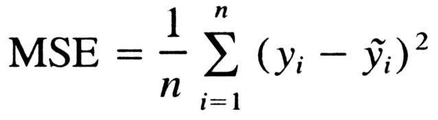
The loss function essentially denotes the error in our prediction. A greater value of the loss function denotes a greater error. Here we will be using Mean Square Error (MSE) as our loss function and it is given by the formula :

损失函数实质上表示我们预测中的误差。 损失函数的值越大表示误差越大。 在这里，我们将使用均方误差(MSE)作为损失函数，它由公式给出：

Once the loss is calculated the we perform an optimization method like gradient descent on the loss function. Stuck with gradient descent, don’t worry, for the time sake all you have to know is that gradient descent is simply a method performed on the loss function to find the values of “w” and “b” that minimizes the loss function. It involves the use of learning rate which can be tweaked for better results. Smaller the loss more accurate is our prediction.

一旦计算出损失，我们就对损失函数执行优化方法，例如梯度下降。 不必担心梯度下降，因为时间上的缘故，您只需要知道梯度下降只是对损失函数执行的一种方法，可以找到使损失函数最小的“ w”和“ b”值。 它涉及学习率的使用，可以对其进行调整以获得更好的结果。 损失越小越准确，这就是我们的预测。

Now what we have seen so far essentially constitutes just one step in the training process. This cycle is repeated a number of times until we arrive at an optimum value of “w” and “b”, where the loss function is minimal.

现在，到目前为止，我们所看到的基本上只是培训过程中的一个步骤。 重复此循环多次，直到我们获得损失函数最小的最佳值“ w”和“ b”。

Okay you have covered the basics of linear regression, now it’s time to code.

好的，您已经介绍了线性回归的基础知识，现在该进行编码了。

线性回归，PyTorch方法 (Linear regression, the PyTorch way)

For simplicity we will be looking at 1D Linear Regression with two parameters. First we import torch for this task.

为简单起见，我们将研究具有两个参数的一维线性回归。 首先，我们为此任务导入火炬。

import torch

The data we will be looking at would be really simple, a torch tensor from -3 to 3 with a step size of 0.1. So lets create our data.

我们将要查看的数据非常简单，步长为0.1的焊炬张量从-3到3。 因此，让我们创建数据。

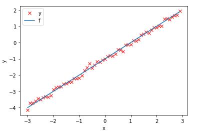
# Create f(X) with a slope of 1 and a bias of -1X = torch.arange(-3, 3, 0.1).view(-1, 1)
f = 1 * X - 1# Add noiseY = f + 0.1 * torch.randn(X.size())

As you might have noticed the equation that our machine wants to learn in this case is y = x -1 where w = 1 and b = -1. Additionally we add some noise to our data so as to make it similar to real world data.

您可能已经注意到，在这种情况下，我们的机器想要学习的方程是y = x -1，其中w = 1和b = -1。 另外，我们在数据中添加了一些噪点，使其与真实世界的数据相似。

A plot of our training set and the function that our machine would like to learn would look like this:

我们的训练集和机器想要学习的功能的图表如下所示：

Now lets create our model and our loss function ( cost function ).

现在让我们创建模型和损失函数(成本函数)。

# Define the forward functiondef forward(x):
    return w * x + b# Define the MSE Loss functiondef criterion(yhat,y):
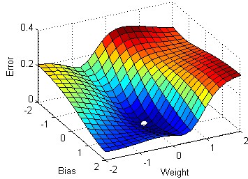
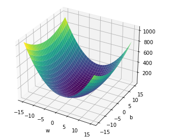
    return torch.mean((yhat-y)**2)

The error surface for the same would look like the figure given below.

相同的错误表面如下图所示。

Now let’s create model parameters w, b by setting the argument requires_grad to True because we must learn it using the data.

现在让我们通过将参数require_grad设置为True来创建模型参数w，b，因为我们必须使用数据来学习它。

# Define the parameters w, b for y = wx + bw = torch.tensor(-15.0, requires_grad = True)
b = torch.tensor(-10.0, requires_grad = True)

Set the learning rate to 0.1 and create an empty list LOSS for storing the loss for each iteration. The LOSS function may be used for plotting and analyzing in the future.

将学习速率设置为0.1，并创建一个空列表LOSS，用于存储每次迭代的损失。 将来可能会使用LOSS功能进行绘图和分析。

# Define learning rate and create an empty list for containing the loss for each iteration.lr = 0.1
LOSS = []

Time to train our model.

是时候训练我们的模型了。

# The function for training the modeldef train_model(iter):
    
    # Loop
    for epoch in range(iter):
        
        # make a prediction
        Yhat = forward(X)
        
        # calculate the loss 
        loss = criterion(Yhat, Y)
            
        # store the loss in the list LOSS
        LOSS.append(loss)
        
        # backward pass
        loss.backward()
        
        # update parameters slope and bias
        w.data = w.data - lr * w.grad.data
        b.data = b.data - lr * b.grad.data
        
        # zero the gradients before running the backward pass
        w.grad.data.zero_()
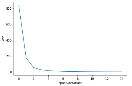
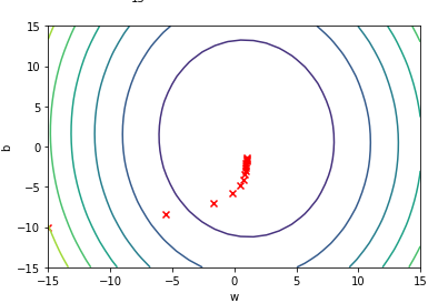
        b.grad.data.zero_()train_model(15)

Here the backward() method computes gradient of the loss with respect to all the learnable parameters. The parameters are updated in each epoch by subtracting from itself the multiple of the gradient and the learning rate . This essentially constitutes the gradient descent method. Feel free to tweak the learning rate, number of epochs and initial value of parameters to get better results.

在这里，backward()方法针对所有可学习的参数计算损耗的梯度。 通过从自身减去梯度和学习率的倍数来更新参数。 这实质上构成了梯度下降法。 随意调整学习率，时期数和参数的初始值以获得更好的结果。

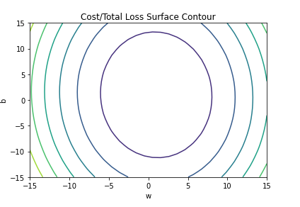
In this case our results would look like this:

在这种情况下，我们的结果将如下所示：

Now let’s see what our model will predict. If we give a value of -3, the output would be y = -3-1 = -4.

现在，让我们看看我们的模型将预测什么。 如果给定值-3，则输出将为y = -3-1 = -4。

x = torch.tensor(-3.)
print(forward(x))#Output
tensor(-4.2857, grad_fn=<AddBackward0>)

Okay we are close enough. Try out different values for the hyper-parameters and we may get interesting results.

好吧，我们已经足够亲密了。 对超参数尝试不同的值，我们可能会得到有趣的结果。

结论 (Conclusion)

Hope you have got an overview of how linear regression works. Good luck learning more about linear regression and other Machine Learning algorithms. Stay hungry Stay Foolish.

希望您对线性回归的工作原理有所了解。 祝您学习有关线性回归和其他机器学习算法的更多信息。 求知若饥，虚怀若愚。