
大模型炼丹术(四):从零开始动手搭建GPT2架构
本文首先搭建GPT架构包含的🧍各个小组件,然后将这些组件串联起来,得到最终的GPT架构。
在前面的3篇文章中,我们已经讲解了训练LLM所需的tokenizer,token/position编码,以及Transformer核心:注意力机制。现在是时候动手搭建GPT的网络架构了。
本文首先搭建GPT架构包含的🧍各个小组件,然后将这些组件串联起来,得到最终的GPT架构。
下图左侧是整个GPT2的架构图,中间是Transformer Block,右侧是我们之前实现的多头注意力层。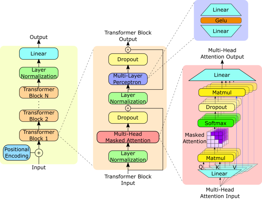
我们要搭建的是GPT-2,具有124M的参数量,相关的配置文件先放这儿:
GPT_CONFIG_124M = {
"vocab_size": 50257,    # Vocabulary size
"context_length": 1024, # Context length
"emb_dim": 768,         # Embedding dimension
"n_heads": 12,          # Number of attention heads
"n_layers": 12,         # Number of layers
"drop_rate": 0.1,       # Dropout rate
"qkv_bias": False# Query-Key-Value bias
}
一、Layer Normalization
1.1 Layer Norm的计算公式
假设某个输入X的batch_size=2,token长度是3,(embedding)的维度是4,如下:
# 定义输入张量 X,形状为 (batch_size=2, seq_len=3, d_model=4)
X = torch.tensor([
    [  # 第一个 batch
        [1.0, 2.0, 3.0, 4.0],
        [5.0, 6.0, 7.0, 8.0],
        [9.0, 10.0, 11.0, 12.0]
    ],
    [  # 第二个 batch
        [13.0, 14.0, 15.0, 16.0],
        [17.0, 18.0, 19.0, 20.0],
        [21.0, 22.0, 23.0, 24å.0]
    ]
])

print(X.shape)  # 输出: torch.Size([2, 3, 4])
接下来以第一个batch为例,讲解LayerNorm层的计算逻辑。
1.1.1 计算均值
LayerNorm 对每个 token(每一行)计算均值:
计算每一行的均值:
所以均值向量为:
1.1.2 计算方差
方差计算公式:
计算每一行的方差:
所以方差向量为:
1.1.3 归一化计算
归一化计算公式:
假设 ( \epsilon = 10^{-5} ),计算标准化后的值:
1.1.4 线性变换(可学习参数)
LayerNorm 通常有两个可训练参数(缩放因子) 和 (偏移量),计算公式为:
假设:
最终的输出:
以上便是第一个batch的LayerNorm计算过程,第二个batch同理。可以看到,LayerNorm是对每一个batch的每一个token对应的维度上进行的,与batch维度无关。
1.2 Transformer中为什么不使用BatchnNorm?
在做图像相关任务时,经常使用Batch Normalization,为什么Transformer中使用的却是Layer Normalization呢?
-
Batch Normalization (BN) 计算的是 batch 维度的均值和方差:
其中,N是 batch 内的样本数,所以它对 batch 之间的分布很敏感。
-
Layer Normalization (LN) 计算的是 每个 token 内的均值和方差(对 embedding 维度归一化):
其中,d是 embedding 维度,即 LN 只依赖于 当前样本自身的信息,不受 batch 影响。
直观理解:
- BN 在图像任务中更常见,因为图像数据通常是 NCHW(batch, channel, height, width)格式,BN 可以在 batch 维度进行统计计算。
- LN 在 NLP、Transformer 结构中更合适,因为序列任务的输入长度不定,且批次大小可能变化,BN 计算的统计量会不稳定。
1.3 Layer Normalization的代码实现
直接将上述的LayerNorm的数学公式用代码实现即可:
import torch.nn as nn
classLayerNorm(nn.Module):
def__init__(self, emb_dim):
        super().__init__()
        self.eps = 1e-5
        self.scale = nn.Parameter(torch.ones(emb_dim))
        self.shift = nn.Parameter(torch.zeros(emb_dim))

defforward(self, x):
        mean = x.mean(dim=-1, keepdim=True)
        var = x.var(dim=-1, keepdim=True, unbiased=False)
        norm_x = (x - mean) / torch.sqrt(var + self.eps)
return self.scale * norm_x + self.shift
实例化测试一下:
batch_example = torch.randn(2, 3, 4)
emb_dim=batch_example.shape[-1]
ln = LayerNorm(emb_dim=4)
out_ln = ln(batch_example)
mean = out_ln.mean(dim=-1, keepdim=True)
var = out_ln.var(dim=-1, unbiased=False, keepdim=True)
print(out_ln.shape)# [2,3,4]
print(mean.shape)# [2,3,1] 每一个token计算一个均值
print(var.shape)# [2,3,1] 每一个token计算一个方差
上面是我们手写的代码。当然,PyTorch中也封装了现成的LayerNorm层,直接调用即可:
layer_norm = torch.nn.LayerNorm(emb_dim)
out_layer_norm = layer_norm(batch_example)
print(out_layer_norm.shape)# [2,3,4]
二、Feed Forward
Feed Forward包括两个线性层和1个GELU激活函数。
2.1 GELU详解
相较于ReLU来说,GELU激活函数具有平滑的性质,因而可以帮助模型更好地学习到非线性关系,且不会像 ReLU 那样因为负输入而使信息完全丢失。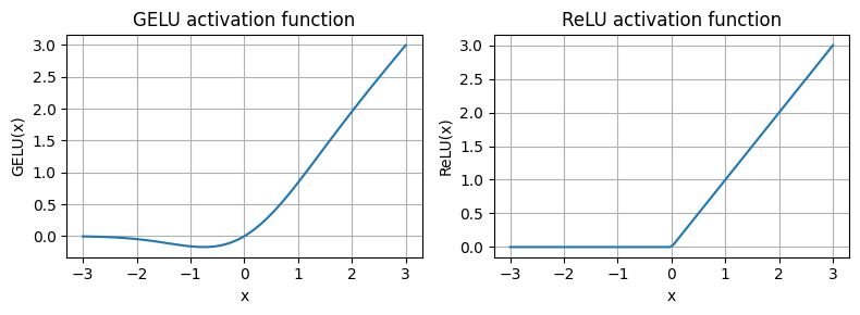
GELU 激活函数的数学表达式为:
π
或者通过高斯误差函数(Error Function, erf)来表示:
根据数学表达式来代码实现GELU:
classGELU(nn.Module):
def__init__(self):
        super().__init__()

defforward(self, x):
return0.5 * x * (1 + torch.tanh(
            torch.sqrt(torch.tensor(2.0 / torch.pi)) *
            (x + 0.044715 * torch.pow(x, 3))
        ))
2.2 Feed Forward的代码实现
classFeedForward(nn.Module):
def__init__(self, cfg):
        super().__init__()
        self.layers = nn.Sequential(
            nn.Linear(cfg["emb_dim"], 4 * cfg["emb_dim"]),
            GELU(),
            nn.Linear(4 * cfg["emb_dim"], cfg["emb_dim"]),
        )

defforward(self, x):
return self.layers(x)
实例化测试一下:
ffn = FeedForward(GPT_CONFIG_124M)
x = torch.rand(2, 3, 768)
out = ffn(x)
print(out.shape)
三、残差连接
残差连接的概念是在CV中提出来的。在深度神经网络中,随着网络层数的加深,梯度可能会在反向传播过程中消失,使得网络的训练变得困难。残差连接允许信息直接流向更深层的网络,而不需要经过每一层的变换,这有助于保留梯度的流动,从而缓解梯度消失问题。换句话说,残差连接通过提供“捷径”路径,确保梯度在训练过程中能够有效传播。
为了进一步说明残差连接对于梯度的影响,这里写一些代码来验证。
首先来定义一个简单的深度神经网络:
classExampleDeepNeuralNetwork(nn.Module):
def__init__(self, layer_sizes, use_shortcut):
        super().__init__()
        self.use_shortcut = use_shortcut
        self.layers = nn.ModuleList([
            nn.Sequential(nn.Linear(layer_sizes[0], layer_sizes[1]), GELU()),
            nn.Sequential(nn.Linear(layer_sizes[1], layer_sizes[2]), GELU()),
            nn.Sequential(nn.Linear(layer_sizes[2], layer_sizes[3]), GELU()),
            nn.Sequential(nn.Linear(layer_sizes[3], layer_sizes[4]), GELU()),
            nn.Sequential(nn.Linear(layer_sizes[4], layer_sizes[5]), GELU())
        ])

defforward(self, x):
for layer in self.layers:
# Compute the output of the current layer
            layer_output = layer(x)
# Check if shortcut can be applied
if self.use_shortcut and x.shape == layer_output.shape:
                x = x + layer_output
else:
                x = layer_output
return x
写一些工具函数,用于查看反向传播时中间层的梯度信息:
defprint_gradients(model, x):
# Forward pass
    output = model(x)
    target = torch.tensor([[0.]])# 假设最后输出的一定是一维

# Calculate loss based on how close the target
# and output are
    loss = nn.MSELoss()
    loss = loss(output, target)

# Backward pass to calculate the gradients
    loss.backward()

for name, param in model.named_parameters():
if'weight'in name:
# Print the mean absolute gradient of the weights
            print(f"{name} has gradient mean of {param.grad.abs().mean().item()}")
不使用残差连接,查看梯度:
layer_sizes = [3, 3, 3, 3, 3, 1]
sample_input = torch.tensor([[1., 0., -1.]])
torch.manual_seed(123) # specify random seed for the initial weights for reproducibility
model_without_shortcut = ExampleDeepNeuralNetwork(
layer_sizes, use_shortcut=False
)

print_gradients(model_without_shortcut, sample_input)
输出:
layers.0.0.weight has gradient mean of 0.00020173587836325169
layers.1.0.weight has gradient mean of 0.00012011159560643137
layers.2.0.weight has gradient mean of 0.0007152039906941354
layers.3.0.weight has gradient mean of 0.0013988736318424344
layers.4.0.weight has gradient mean of 0.005049645435065031
不使用残差连接,查看梯度:
torch.manual_seed(123)
model_with_shortcut = ExampleDeepNeuralNetwork(
layer_sizes, use_shortcut=True
)
print_gradients(model_with_shortcut, sample_input)
输出:
layers.0.0.weight has gradient mean of 0.22169792652130127
layers.1.0.weight has gradient mean of 0.20694106817245483
layers.2.0.weight has gradient mean of 0.32896995544433594
layers.3.0.weight has gradient mean of 0.2665732204914093
layers.4.0.weight has gradient mean of 1.3258540630340576
使用残差连接后,即使是最靠近输入的网络层的梯度仍维持在0.22左右,远大于不使用残差连接的时0.00002。
在我们要实现的GPT-2架构中,主要有两个部分用到了残差连接: 1)自注意力层的残差连接 2)前馈网络的残差连接
这些将体现在后面的代码中,请继续往下看。
四、编写Transformer Block
有了前面三部分的组件,就可以将它们合起来构建Transformer Block了。
现在来代码实现中间的Transformer Block:
classTransformerBlock(nn.Module):
def__init__(self, cfg):
        super().__init__()
        self.att = MultiHeadAttention(
            d_in=cfg["emb_dim"],
            d_out=cfg["emb_dim"],
            context_length=cfg["context_length"],
            num_heads=cfg["n_heads"],
            dropout=cfg["drop_rate"],
            qkv_bias=cfg["qkv_bias"])
        self.ff = FeedForward(cfg)
        self.norm1 = LayerNorm(cfg["emb_dim"])
        self.norm2 = LayerNorm(cfg["emb_dim"])
        self.drop_shortcut = nn.Dropout(cfg["drop_rate"])

defforward(self, x):
# Shortcut connection for attention block
        shortcut = x
        x = self.norm1(x)
        x = self.att(x)  # Shape [batch_size, num_tokens, emb_size]
        x = self.drop_shortcut(x)
        x = x + shortcut  # Add the original input back

# Shortcut connection for feed forward block
        shortcut = x
        x = self.norm2(x)
        x = self.ff(x)
        x = self.drop_shortcut(x)
        x = x + shortcut  # Add the original input back

return x
实例化测试一下:
import torch
x = torch.rand(2, 4, 768) #A
block = TransformerBlock(GPT_CONFIG_124M)
output = block(x)
print("Input shape:", x.shape)# [2, 4, 768]
print("Output shape:", output.shape)# [2, 4, 768]
五、编写整个GPT2架构
本小节将实现左图的GPT2架构
现在所有组件都有了,直接根据上面左侧的架构图串联起来就好了:
classGPTModel(nn.Module):
def__init__(self, cfg):
        super().__init__()
        self.tok_emb = nn.Embedding(cfg["vocab_size"], cfg["emb_dim"])
        self.pos_emb = nn.Embedding(cfg["context_length"], cfg["emb_dim"])
        self.drop_emb = nn.Dropout(cfg["drop_rate"])

        self.trf_blocks = nn.Sequential(
            *[TransformerBlock(cfg) for _ in range(cfg["n_layers"])])

        self.final_norm = LayerNorm(cfg["emb_dim"])
        self.out_head = nn.Linear(
            cfg["emb_dim"], cfg["vocab_size"], bias=False
        )

defforward(self, in_idx):
        batch_size, seq_len = in_idx.shape
# tok_embeds: [2, 4, 768]
        tok_embeds = self.tok_emb(in_idx)
# pos_embeds: [4, 768]
        pos_embeds = self.pos_emb(torch.arange(seq_len, device=in_idx.device))
# x Shape: [batch_size, num_tokens, emb_size]
        x = tok_embeds + pos_embeds# x Shape:[2,4,768]
        x = self.drop_emb(x)
        x = self.trf_blocks(x)
        x = self.final_norm(x)
        logits = self.out_head(x)
return logits
实例化测试:
torch.manual_seed(123)
model = GPTModel(GPT_CONFIG_124M)
out = model(batch)
print(batch)# tensor([[6109, 3626, 6100,  345],
#          [6109, 1110, 6622,  257]])
print("Input batch:", batch.shape)# [2,4],batch_size是2,每个batch的句子包含4个token
print("Output shape:", out.shape)# [2,4,50257]# 词表的长度是50257
到这里,我们完成了整个GPT2架构的搭建。
六、使用GPT进行逐个token预测
在使用类似ChatGPT等LLM时,生成的对话是一种形如打字机效果来展示的,事实上,LLM在推理过程中也是自回归地逐个token预测的,这与其 Transformer Decoder 结构和 因果注意力(Causal Attention) 机制有关。
预测下一个单词的函数代码如下:
defgenerate_text_simple(model, idx, max_new_tokens, context_size):
# idx 是 (batch, n_tokens) 形状的张量,表示当前上下文中的 Token 索引
for _ in range(max_new_tokens):

# 如果当前上下文长度超过模型支持的最大长度,则进行截断
# 例如,如果 LLM 只能支持 5 个 Token,而当前上下文长度是 10
# 那么只保留最后 5 个 Token 作为输入
        idx_cond = idx[:, -context_size:]

# 获取模型的预测结果
with torch.no_grad():  # 关闭梯度计算,加速推理
            logits = model(idx_cond)  # (batch, n_tokens, vocab_size)

# 只关注最后一个时间步的预测结果
# (batch, n_tokens, vocab_size) 变为 (batch, vocab_size)
        logits = logits[:, -1, :]

# 通过 Softmax 计算概率分布,后续文章将介绍其他方式
        probas = torch.softmax(logits, dim=-1)  # (batch, vocab_size)

# 选择概率最高的 Token 作为下一个 Token
        idx_next = torch.argmax(probas, dim=-1, keepdim=True)  # (batch, 1)

# 将新生成的 Token 追加到序列中
        idx = torch.cat((idx, idx_next), dim=1)  # (batch, n_tokens+1)

return idx  # 返回完整的 Token 序列
原来很简单,假设初始的输入token序列长度是4,每预测一个token,就把预测得到的token拼接在初始token后面,作为新的输入token序列。
来实例化测试一下。
首先使用tokenizer将已有文本start_context编码到token id的形式
start_context = "Hello, I am"
encoded = tokenizer.encode(start_context)
print("encoded:", encoded)
encoded_tensor = torch.tensor(encoded).unsqueeze(0) #A
print("encoded_tensor.shape:", encoded_tensor.shape)
输出:
encoded: [15496, 11, 314, 716]
encoded_tensor.shape: torch.Size([1, 4])
然后调用上面的生成函数generate_text_simple,开始自回归地预测下一个单词
model.eval() #A
out = generate_text_simple(
model=model,
idx=encoded_tensor,
max_new_tokens=6,
context_size=GPT_CONFIG_124M["context_length"]
)
print("Output:", out)
print("Output length:", len(out[0]))
输出:
Output: tensor([[15496,    11,   314,   716, 27018, 24086, 47843, 30961, 42348,  7267]])
Output length: 10
预测完成后,使用tokenizer的decode方法,将预测的token还原成文本:
decoded_text = tokenizer.decode(out.squeeze(0).tolist())
print(decoded_text)# Hello, I am Featureiman Byeswickattribute argue
可以看到,模型的预测已经被解码成文本的形式,但是你会发现,虽然已经拿到了预测结果,读起来却明显是不通顺的。
这是因为模型还没有经过训练,我们当前测试的GPT2的权重是随机初始化的。在接下来的文章中,我们将介绍如何对GPT2进行训练,以生成有意义的可读文本,并通过一系列技术手段进行逐步优化,欢迎持续关注。
大模型算是目前当之无愧最火的一个方向了,算是新时代的风口!有小伙伴觉得,作为新领域、新方向人才需求必然相当大,与之相应的人才缺乏、人才竞争自然也会更少,那转行去做大模型是不是一个更好的选择呢?是不是更好就业呢?是不是就暂时能抵抗35岁中年危机呢?
答案当然是这样,大模型必然是新风口!
那如何学习大模型 ?
由于新岗位的生产效率,要优于被取代岗位的生产效率,所以实际上整个社会的生产效率是提升的。但是具体到个人,只能说是:
最先掌握AI的人,将会比较晚掌握AI的人有竞争优势。
这句话,放在计算机、互联网、移动互联网的开局时期,都是一样的道理。
但现在很多想入行大模型的人苦于现在网上的大模型老课程老教材,学也不是不学也不是,基于此我用做产品的心态来打磨这份大模型教程,深挖痛点并持续修改了近100余次后,终于把整个AI大模型的学习路线完善出来!

在这个版本当中:
您只需要听我讲,跟着我做即可,为了让学习的道路变得更简单,这份大模型路线+学习教程已经给大家整理并打包分享出来, 😝有需要的小伙伴,可以 扫描下方二维码领取🆓↓↓↓

一、大模型经典书籍(免费分享)
AI大模型已经成为了当今科技领域的一大热点,那以下这些大模型书籍就是非常不错的学习资源。

二、640套大模型报告(免费分享)
这套包含640份报告的合集,涵盖了大模型的理论研究、技术实现、行业应用等多个方面。无论您是科研人员、工程师,还是对AI大模型感兴趣的爱好者,这套报告合集都将为您提供宝贵的信息和启示。(几乎涵盖所有行业)
三、大模型系列视频教程(免费分享)

四、2025最新大模型学习路线(免费分享)
我们把学习路线分成L1到L4四个阶段,一步步带你从入门到进阶,从理论到实战。
L1阶段:启航篇丨极速破界AI新时代
L1阶段:了解大模型的基础知识,以及大模型在各个行业的应用和分析,学习理解大模型的核心原理、关键技术以及大模型应用场景。
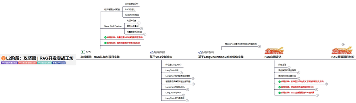
L2阶段:攻坚篇丨RAG开发实战工坊
L2阶段:AI大模型RAG应用开发工程,主要学习RAG检索增强生成:包括Naive RAG、Advanced-RAG以及RAG性能评估,还有GraphRAG在内的多个RAG热门项目的分析。
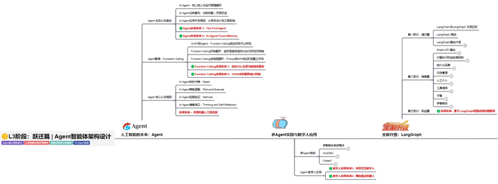
L3阶段:跃迁篇丨Agent智能体架构设计
L3阶段:大模型Agent应用架构进阶实现,主要学习LangChain、 LIamaIndex框架,也会学习到AutoGPT、 MetaGPT等多Agent系统,打造Agent智能体。
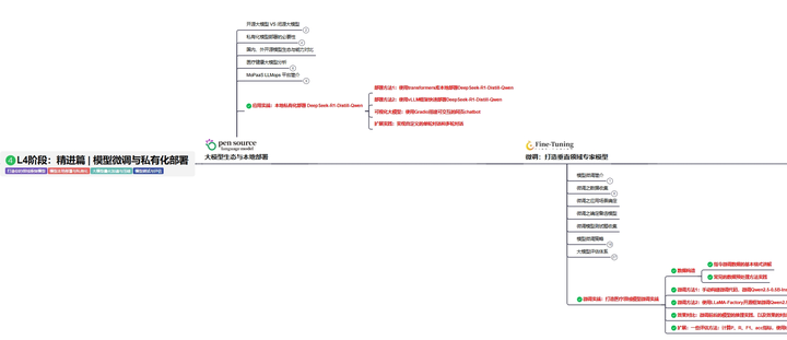
L4阶段:精进篇丨模型微调与私有化部署
L4阶段:大模型的微调和私有化部署,更加深入的探讨Transformer架构,学习大模型的微调技术,利用DeepSpeed、Lamam Factory等工具快速进行模型微调,并通过Ollama、vLLM等推理部署框架,实现模型的快速部署。
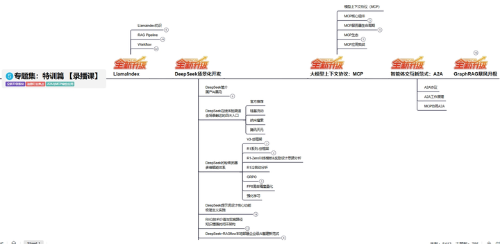
L5阶段:专题集丨特训篇 【录播课】
全套的AI大模型学习资源已经整理打包,有需要的小伙伴可以微信扫描下方二维码,免费领取
更多推荐


 9
9 0
0- 0


 已为社区贡献12条内容

所有评论(0)