数据集划分

先将数据集划分为训练集、验证集和测试集，标记为X,y、Xval,yval和Xtest,ytest。关于数据集划分的内容可看这篇博客。

数据可视化

吴恩达作业常规第一步，数据可视化，这里只可视化了训练集：

% Load from ex5data1: 
% You will have X, y, Xval, yval, Xtest, ytest in your environment
load ('ex5data1.mat');
% m = Number of examples
m = size(X, 1);

% Plot training data
figure;
plot(X, y, 'rx', 'MarkerSize', 10, 'LineWidth', 1.5);
xlabel('Change in water level (x)');
ylabel('Water flowing out of the dam (y)');

代价-梯度函数

线性回归算是最基础的机器学习算法了，它的代价和梯度的公式相信大🔥也不陌生，代价函数为
$$J(\theta )=\frac{1}{2m}\sum _{i=1}^m({\theta }_0{x}_0^{(i)}+{\theta }_1{x}_1^{(i)}+\cdots +{\theta }_n{x}_n^{(i)}-y^{(i)}{)}^2+\frac{\lambda }{2m}\sum _{j=1}^n{\theta }_j^2$$
梯度为
$$\frac{\partial J(\theta )}{\partial {\theta }_j}=\frac{1}{m}\sum _{i=1}^m{x}_j^{(i)}({\theta }_0{x}_0^{(i)}+{\theta }_1{x}_1^{(i)}+\cdots +{\theta }_n{x}_n^{(i)}-y^{(i)})+\frac{\lambda }{m}{\theta }_j$$
向量化过程也蛮简单的，注意一下${\theta }_0$不参与正则化就好，我就直接上代码了：

function [J, grad] = linearRegCostFunction(X, y, theta, lambda)
%LINEARREGCOSTFUNCTION Compute cost and gradient for regularized linear 
%regression with multiple variables
%   [J, grad] = LINEARREGCOSTFUNCTION(X, y, theta, lambda) computes the 
%   cost of using theta as the parameter for linear regression to fit the 
%   data points in X and y. Returns the cost in J and the gradient in grad

% Initialize some useful values
m = length(y); % number of training examples

% You need to return the following variables correctly 
J = 0;
grad = zeros(size(theta));

% ====================== YOUR CODE HERE ======================
% Instructions: Compute the cost and gradient of regularized linear 
%               regression for a particular choice of theta.
%
%               You should set J to the cost and grad to the gradient.
%

h=X*theta;
J=sum((h-y).^2)/(2*m);
J=J+(lambda/(2*m))*(sum(theta.^2)-theta(1)^2);

grad=X'*(h-y)/m;
tmp=grad(1);
grad=grad+(lambda/m)*theta;
grad(1)=tmp;

% =========================================================================

grad = grad(:);

end

求解

求解过程很简单，调用我们写的代价-梯度函数即可，吴恩达直接提供了代码：

function [theta] = trainLinearReg(X, y, lambda)
%TRAINLINEARREG Trains linear regression given a dataset (X, y) and a
%regularization parameter lambda
%   [theta] = TRAINLINEARREG (X, y, lambda) trains linear regression using
%   the dataset (X, y) and regularization parameter lambda. Returns the
%   trained parameters theta.
%

% Initialize Theta
initial_theta = zeros(size(X, 2), 1); 

% Create "short hand" for the cost function to be minimized
costFunction = @(t) linearRegCostFunction(X, y, t, lambda);

% Now, costFunction is a function that takes in only one argument
options = optimset('MaxIter', 200, 'GradObj', 'on');

% Minimize using fmincg
theta = fmincg(costFunction, initial_theta, options);

end

线性拟合

首先我们尝试用一根直线（一个特征值两个参数）去拟合，肯定效果不咋地，这是结果：

绘制学习曲线

显然上面出现的是欠拟合问题，我们可以通过它的学习曲线来确认这一判断。计算训练代价和验证代价的函数与代价函数基本相同，但不包含正则项。然后边改变训练集大小边计算代价即可：

function [error_train, error_val] = ...
    learningCurve(X, y, Xval, yval, lambda)
%LEARNINGCURVE Generates the train and cross validation set errors needed 
%to plot a learning curve
%   [error_train, error_val] = ...
%       LEARNINGCURVE(X, y, Xval, yval, lambda) returns the train and
%       cross validation set errors for a learning curve. In particular, 
%       it returns two vectors of the same length - error_train and 
%       error_val. Then, error_train(i) contains the training error for
%       i examples (and similarly for error_val(i)).
%
%   In this function, you will compute the train and test errors for
%   dataset sizes from 1 up to m. In practice, when working with larger
%   datasets, you might want to do this in larger intervals.
%

% Number of training examples
m = size(X, 1);

% You need to return these values correctly
error_train = zeros(m, 1);
error_val   = zeros(m, 1);

% ====================== YOUR CODE HERE ======================
% Instructions: Fill in this function to return training errors in 
%               error_train and the cross validation errors in error_val. 
%               i.e., error_train(i) and 
%               error_val(i) should give you the errors
%               obtained after training on i examples.
%
% Note: You should evaluate the training error on the first i training
%       examples (i.e., X(1:i, :) and y(1:i)).
%
%       For the cross-validation error, you should instead evaluate on
%       the _entire_ cross validation set (Xval and yval).
%
% Note: If you are using your cost function (linearRegCostFunction)
%       to compute the training and cross validation error, you should 
%       call the function with the lambda argument set to 0. 
%       Do note that you will still need to use lambda when running
%       the training to obtain the theta parameters.
%
% Hint: You can loop over the examples with the following:
%
%       for i = 1:m
%           % Compute train/cross validation errors using training examples 
%           % X(1:i, :) and y(1:i), storing the result in 
%           % error_train(i) and error_val(i)
%           ....
%           
%       end
%

% ---------------------- Sample Solution ----------------------

for i=1:m
    tmpX=X(1:i,:);
    tmpy=y(1:i);
    [theta]=trainLinearReg(tmpX, tmpy, lambda);
    [error_train(i)]=linearRegCostFunction(tmpX,tmpy,theta,0);
    [error_val(i)]=linearRegCostFunction(Xval,yval,theta,0);
end




% -------------------------------------------------------------

% =========================================================================

end

lambda = 0;
[error_train, error_val] = learningCurve([ones(m, 1) X], y, [ones(size(Xval, 1), 1) Xval], yval, lambda);

plot(1:m, error_train, 1:m, error_val);
title('Learning curve for linear regression')
legend('Train', 'Cross Validation')
xlabel('Number of training examples')
ylabel('Error')
axis([0 13 0 150])

更好的方法是，从训练集中随机选择示例，并从交叉验证集中随机选择示例。然后，使用随机选择的训练集学习参数，并在随机选择的训练集和交叉验证集上评估参数。重复上述步骤多次（比如 50 次），使用平均误差来确定示例的训练误差和交叉验证误差，这样可以得到更平滑的曲线。

多项式拟合

显然，我们并不能满足于用一条直线去拟合，我们应该尝试用多项式，使用多项式拟合时还要用到特征缩放。特征缩放在ex1已经实现过类似的了，这里吴恩达提供的代码也是类似，但是调用了高级函数：

function [X_norm, mu, sigma] = featureNormalize(X)
%FEATURENORMALIZE Normalizes the features in X 
%   FEATURENORMALIZE(X) returns a normalized version of X where
%   the mean value of each feature is 0 and the standard deviation
%   is 1. This is often a good preprocessing step to do when
%   working with learning algorithms.

mu = mean(X);
X_norm = bsxfun(@minus, X, mu);

sigma = std(X_norm);
X_norm = bsxfun(@rdivide, X_norm, sigma);


% ============================================================

end

我们实现的是生成高次项的函数：

function [X_poly] = polyFeatures(X, p)
%POLYFEATURES Maps X (1D vector) into the p-th power
%   [X_poly] = POLYFEATURES(X, p) takes a data matrix X (size m x 1) and
%   maps each example into its polynomial features where
%   X_poly(i, :) = [X(i) X(i).^2 X(i).^3 ...  X(i).^p];
%


% You need to return the following variables correctly.
X_poly = zeros(numel(X), p);

% ====================== YOUR CODE HERE ======================
% Instructions: Given a vector X, return a matrix X_poly where the p-th 
%               column of X contains the values of X to the p-th power.
%
% 

for i=1:p
    X_poly(:,i)=X.^i;
end



% =========================================================================

end

p = 8;

% Map X onto Polynomial Features and Normalize
X_poly = polyFeatures(X, p);
[X_poly, mu, sigma] = featureNormalize(X_poly);  % Normalize
X_poly = [ones(m, 1), X_poly];                   % Add Ones

% Map X_poly_test and normalize (using mu and sigma)
X_poly_test = polyFeatures(Xtest, p);
X_poly_test = X_poly_test-mu; % uses implicit expansion instead of bsxfun
X_poly_test = X_poly_test./sigma; % uses implicit expansion instead of bsxfun
X_poly_test = [ones(size(X_poly_test, 1), 1), X_poly_test];         % Add Ones

% Map X_poly_val and normalize (using mu and sigma)
X_poly_val = polyFeatures(Xval, p);
X_poly_val = X_poly_val-mu; % uses implicit expansion instead of bsxfun
X_poly_val = X_poly_val./sigma; % uses implicit expansion instead of bsxfun
X_poly_val = [ones(size(X_poly_val, 1), 1), X_poly_val];           % Add Ones

fprintf('Normalized Training Example 1:\n');

再次求解

% Train the model
lambda = 0;
[theta] = trainLinearReg(X_poly, y, lambda);
% Plot training data and fit
plot(X, y, 'rx', 'MarkerSize', 10, 'LineWidth', 1.5);
plotFit(min(X), max(X), mu, sigma, theta, p);
xlabel('Change in water level (x)');
ylabel('Water flowing out of the dam (y)');
title (sprintf('Polynomial Regression Fit (lambda = %f)', lambda));

因为这里正则参数$\lambda$设置为0，显然我们的模型过拟合了：

从它的学习曲线也可以判断这一点：

plot(1:m, error_train, 1:m, error_val);
title(sprintf('Polynomial Regression Learning Curve (lambda = %f)', lambda));
xlabel('Number of training examples')
ylabel('Error')
axis([0 13 0 100])
legend('Train', 'Cross Validation')

可以看到我们的训练误差一直是0，但是验证误差并不小。

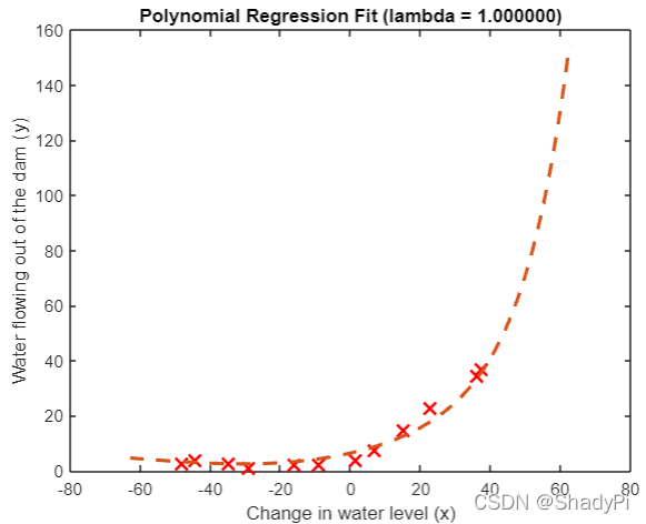
将$\lambda$设置为1，可以明显看到拟合改善：

% Choose the value of lambda
lambda = 1;
[theta] = trainLinearReg(X_poly, y, lambda);

% Plot training data and fit
plot(X, y, 'rx', 'MarkerSize', 10, 'LineWidth', 1.5);
plotFit(min(X), max(X), mu, sigma, theta, p);
xlabel('Change in water level (x)');
ylabel('Water flowing out of the dam (y)');
title (sprintf('Polynomial Regression Fit (lambda = %f)', lambda));

plot(1:m, error_train, 1:m, error_val);
title(sprintf('Polynomial Regression Learning Curve (lambda = %f)', lambda));
xlabel('Number of training examples')
ylabel('Error')
axis([0 13 0 100])
legend('Train', 'Cross Validation')

将$\lambda$改为100，问题又出现了，很明显我们欠拟合得离谱：


那么我们究竟该如何选择正则参数呢，有没有比1更好的$\lambda$？

选择合适的正则参数

我们可以采用划分训练集、验证集、测试集的方法，先列出一系列$\lambda$，在训练集中训练，得到模型放到验证集中看谁最优秀，把最优秀的拿到测试集中试一试是否过拟合。

function [lambda_vec, error_train, error_val] = ...
    validationCurve(X, y, Xval, yval)
%VALIDATIONCURVE Generate the train and validation errors needed to
%plot a validation curve that we can use to select lambda
%   [lambda_vec, error_train, error_val] = ...
%       VALIDATIONCURVE(X, y, Xval, yval) returns the train
%       and validation errors (in error_train, error_val)
%       for different values of lambda. You are given the training set (X,
%       y) and validation set (Xval, yval).
%

% Selected values of lambda (you should not change this)
lambda_vec = [0 0.001 0.003 0.01 0.03 0.1 0.3 1 3 10]';

% You need to return these variables correctly.
error_train = zeros(length(lambda_vec), 1);
error_val = zeros(length(lambda_vec), 1);

% ====================== YOUR CODE HERE ======================
% Instructions: Fill in this function to return training errors in 
%               error_train and the validation errors in error_val. The 
%               vector lambda_vec contains the different lambda parameters 
%               to use for each calculation of the errors, i.e, 
%               error_train(i), and error_val(i) should give 
%               you the errors obtained after training with 
%               lambda = lambda_vec(i)
%
% Note: You can loop over lambda_vec with the following:
%
%       for i = 1:length(lambda_vec)
%           lambda = lambda_vec(i);
%           % Compute train / val errors when training linear 
%           % regression with regularization parameter lambda
%           % You should store the result in error_train(i)
%           % and error_val(i)
%           ....
%           
%       end
%
%
for i=1:length(lambda_vec)
    lambda=lambda_vec(i);
    [theta]=trainLinearReg(X, y, lambda);
    [error_train(i)]=linearRegCostFunction(X,y,theta,0);
    [error_val(i)]=linearRegCostFunction(Xval,yval,theta,0);
end

% =========================================================================

end

按照这样的做法，我们可以得到一条代价-$\lambda$曲线：

可以发现，在$\lambda =3$时验证代价最小，放到测试集里试一试：

lambda=3;
[theta]=trainLinearReg(X_poly, y, lambda);
fprintf("%f\n",linearRegCostFunction(X_poly_test,ytest,theta,0));

代价为3.8599，说明我们的拟合还是相当合适的。