第五章-自己搭建大模型_第1部分-动手实现一个LLaMA2大模型

总目录

1. 第一章 NLP基础概念完整指南

   1. 第1部分-概念和发展历史
   2. 第2部分-各种任务（实体识别、关系抽取、文本摘要、机器翻译、自动问答）
   3. 第3部分-文本表示（词向量、语言模型、ELMo）

2. 第二章 Transformer 架构原理

   1. 第1部分-注意力机制
   2. 第2部分Encoder-Decoder架构
   3. 第3部分-完整Transformer模型）

3. 第三章 预训练语言模型

   1. 第1部分-Encoder-only（BERT、RoBERTa、ALBERT）
   2. 第2部分-Encoder-Decoder-T5
   3. 第3部分-Decoder-Only（GPT、LLama、GLM）

4. 第四章 大语言模型

   1. 第1部分-发展历程、上下文、指令遵循、多模态
   2. 第2部分-LLM预训练、监督微调、强化学习

5. 第五章 动手搭建大模型

   1. 第1部分-动手实现一个LLaMA2大模型
   2. 第2部分-自己训练 Tokenizer
   3. 第3部分-预训练一个小型LLM

6. 第六章 大模型训练实践

   1. 第1部分-模型预训练
   2. 第2部分-模型有监督微调
   3. 第3部分-高效微调

7. 第七章 大模型实战

   1. 第1部分-评测+RAG检索增强生成
   2. 第2部分-智能体Agent系统

目录

1. 动手实现一个 LLaMA2 大模型
   • 1.1 定义超参数
   • 1.2 构建 RMSNorm
   • 1.3 构建 LLaMA2 Attention
   • 1.4 构建 LLaMA2 MLP模块
   • 1.5 构建 LLaMA2 Decoder Layer
   • 1.6 构建完整的 LLaMA2 模型

---

1. 动手实现一个 LLaMA2 大模型

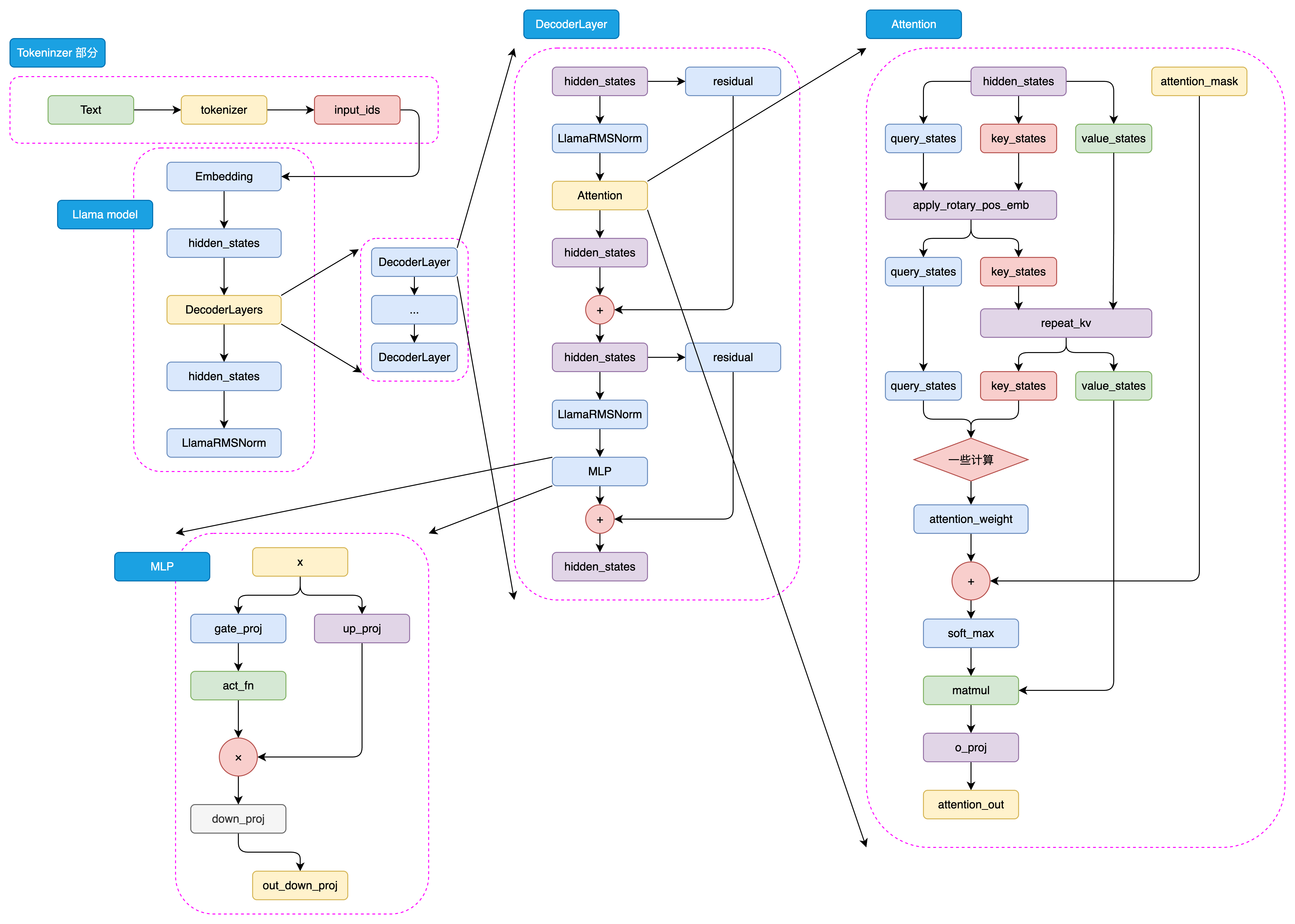
Meta公司在2023年2月发布了LLaMA（Large Language Model Meta AI），并在7月推出了升级版LLaMA2。LLaMA2采用了decoder-only的Transformer架构，在保持高性能的同时，通过一系列优化（如RMSNorm、RoPE、GQA等）提升了训练效率和推理速度。

本章将手把手带你实现一个完整的LLaMA2模型，从最基础的归一化层到最终的文本生成，让你真正理解大模型的每一个细节。

1.1 定义超参数

在开始编写代码之前，我们需要先定义模型的超参数配置。超参数决定了模型的规模和能力上限，合理的超参数设置是训练成功的第一步。

from transformers import PretrainedConfig

class ModelConfig(PretrainedConfig):
    """
    LLaMA2模型配置类
    继承自PretrainedConfig以便与HuggingFace生态兼容
    """
    model_type = "Tiny-K"
    
    def __init__(
        self,
        dim: int = 768,              # 模型隐藏层维度
        n_layers: int = 12,          # Transformer层数
        n_heads: int = 16,           # 注意力头数
        n_kv_heads: int = 8,         # 键值头数（用于GQA）
        vocab_size: int = 6144,      # 词表大小
        hidden_dim: int = None,      # FFN隐藏层维度
        multiple_of: int = 64,       # FFN维度的倍数约束
        norm_eps: float = 1e-5,      # 归一化层的epsilon
        max_seq_len: int = 512,      # 最大序列长度
        dropout: float = 0.0,        # Dropout概率
        flash_attn: bool = True,     # 是否使用Flash Attention
        **kwargs,
    ):
        self.dim = dim
        self.n_layers = n_layers
        self.n_heads = n_heads
        self.n_kv_heads = n_kv_heads
        self.vocab_size = vocab_size
        self.hidden_dim = hidden_dim
        self.multiple_of = multiple_of
        self.norm_eps = norm_eps
        self.max_seq_len = max_seq_len
        self.dropout = dropout
        self.flash_attn = flash_attn
        super().__init__(**kwargs)

关键参数解读：

• dim (模型维度)：控制模型的表达能力，常见值有768、1024、2048等。更大的维度意味着更强的表达能力，但也需要更多显存。

• n_layers (层数)：决定模型的深度。LLaMA2-7B使用32层，我们的小模型使用12-18层。

• n_heads (注意力头数)：多头注意力机制中的头数，必须能整除dim。更多的头可以学习到更丰富的特征模式。

• n_kv_heads (键值头数)：GQA（分组查询注意力）的关键参数。当n_kv_heads < n_heads时，多个查询头共享同一组键值头，可以显著降低显存占用和提升推理速度。

• max_seq_len (最大序列长度)：模型能处理的最长文本长度。受限于显存和位置编码设计，训练时需要合理设置。

1.2 构建 RMSNorm

RMSNorm（Root Mean Square Layer Normalization）是LLaMA系列模型的重要创新之一。相比传统的LayerNorm，它省去了计算均值和减去均值的操作，在保持归一化效果的同时提升了计算效率。

数学原理：

传统LayerNorm的公式为：

$$\text{LayerNorm}(x)=\frac{x-\mu }{\sqrt{{\sigma }^2+ϵ}}\cdot \gamma +\beta$$

RMSNorm简化为：

$$\text{RMSNorm}(x)=\frac{x}{\text{RMS}(x)}\cdot \gamma =\frac{x}{\sqrt{\frac{1}{n}{\sum }_{i=1}^n{x}_i^2+ϵ}}\cdot \gamma$$

其中：

• $x_i$ 是输入向量的第 $i$ 个元素
• $n$ 是向量维度
• $ϵ$ 是防止除零的小常数（通常为 $10^{-5}$ 或 $10^{-6}$）
• $\gamma$ 是可学习的缩放参数

代码实现：

import torch
import torch.nn as nn

class RMSNorm(nn.Module):
    """
    RMS Layer Normalization
    相比LayerNorm去除了均值中心化，计算更高效
    """
    def __init__(self, dim: int, eps: float = 1e-5):
        super().__init__()
        self.eps = eps  # 防止除零
        self.weight = nn.Parameter(torch.ones(dim))  # 可学习的缩放因子

    def _norm(self, x):
        """
        计算RMS归一化
        x: [batch_size, seq_len, dim]
        """
        # 计算平方的均值，然后取平方根的倒数
        rms = torch.rsqrt(x.pow(2).mean(-1, keepdim=True) + self.eps)
        return x * rms

    def forward(self, x):
        """
        前向传播
        保证数值稳定性：先转float32计算，再转回原类型
        """
        output = self._norm(x.float()).type_as(x)
        return output * self.weight

为什么RMSNorm有效？

RMSNorm的核心思想是：归一化的主要作用是控制激活值的规模，而均值中心化并非必需。通过RMS归一化，可以：

1. 将激活值缩放到合理范围
2. 稳定梯度传播
3. 加速训练收敛

实验表明，RMSNorm在大多数任务上与LayerNorm效果相当，但计算速度提升约7-10%。

测试代码：

# 创建RMSNorm实例
args = ModelConfig()
norm = RMSNorm(args.dim, args.norm_eps)

# 生成随机输入
x = torch.randn(2, 50, args.dim)  # [batch_size, seq_len, dim]
output = norm(x)

print(f"输入形状: {x.shape}")
print(f"输出形状: {output.shape}")
print(f"归一化前均值: {x.mean(-1)[0, 0]:.4f}, 标准差: {x.std(-1)[0, 0]:.4f}")
print(f"归一化后均值: {output.mean(-1)[0, 0]:.4f}, 标准差: {output.std(-1)[0, 0]:.4f}")

# 输出示例：
# 输入形状: torch.Size([2, 50, 768])
# 输出形状: torch.Size([2, 50, 768])
# 归一化前均值: -0.0234, 标准差: 1.0123
# 归一化后均值: -0.0234, 标准差: 0.9987

可以看到，RMSNorm保持了输入的形状，并有效地稳定了数值分布。

1.3 构建 LLaMA2 Attention

注意力机制是Transformer的核心。LLaMA2采用了分组查询注意力（Grouped-Query Attention, GQA），这是介于多头注意力（MHA）和多查询注意力（MQA）之间的一种折中方案。

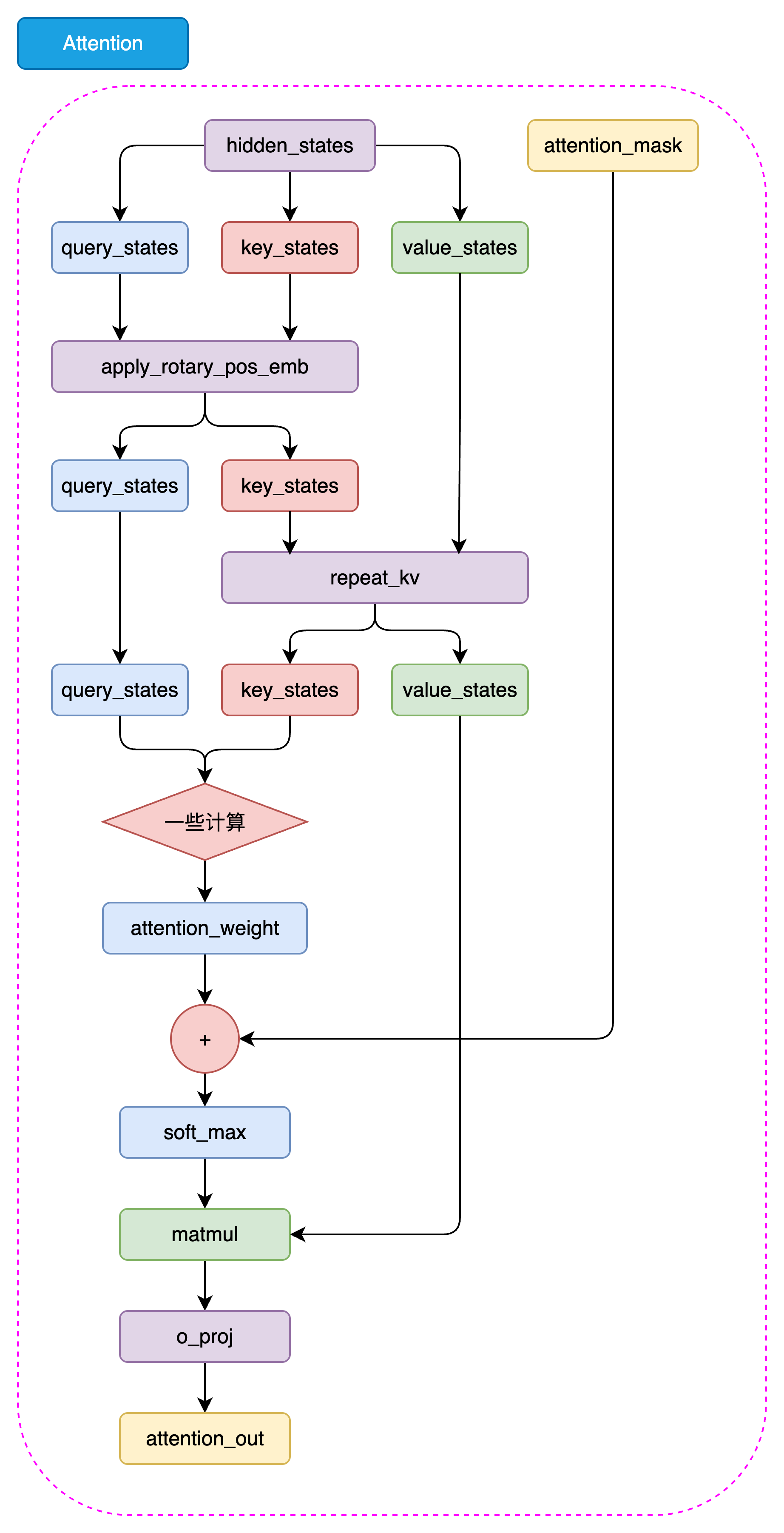
GQA工作原理：

• MHA（Multi-Head Attention）：每个查询头都有对应的键值头，参数量大但效果好
• MQA（Multi-Query Attention）：所有查询头共享一组键值头，参数量小但可能损失性能
• GQA：将查询头分组，每组共享键值头，平衡了参数量和性能

假设有8个查询头和2个键值头，则4个查询头共享1个键值头。

1.3.1 repeat_kv 函数

def repeat_kv(x: torch.Tensor, n_rep: int) -> torch.Tensor:
    """
    将键值头复制n_rep次以匹配查询头数量
    
    Args:
        x: [batch_size, seq_len, n_kv_heads, head_dim]
        n_rep: 每个键值头需要复制的次数
        
    Returns:
        [batch_size, seq_len, n_kv_heads * n_rep, head_dim]
    """
    bs, slen, n_kv_heads, head_dim = x.shape
    
    if n_rep == 1:
        return x
    
    # 在第4个维度插入新维度并扩展
    return (
        x[:, :, :, None, :]  # [bs, slen, n_kv_heads, 1, head_dim]
        .expand(bs, slen, n_kv_heads, n_rep, head_dim)
        .reshape(bs, slen, n_kv_heads * n_rep, head_dim)
    )

1.3.2 旋转位置编码（RoPE）

RoPE（Rotary Position Embedding）是LLaMA的另一创新。传统位置编码将位置信息直接加到token嵌入上，而RoPE通过旋转的方式将位置信息编码到注意力机制中。

核心思想：

将query和key视为复数，通过旋转角度来编码相对位置信息。对于位置m的向量和位置n的向量，它们的内积会包含(m-n)的信息，从而实现相对位置编码。

数学推导：

对于第$m$个位置的向量$q_m$和第$n$个位置的向量$k_n$，经过RoPE后：

$q_m=R_{\Theta ,m}\cdot x_m,k_n=R_{\Theta ,n}\cdot x_n$

其中$R_{\Theta ,m}$是旋转矩阵。两者的内积为：

$⟨q_m,k_n⟩=x_m^T{R}_{\Theta ,m}^T{R}_{\Theta ,n}{x}_n=x_m^T{R}_{\Theta ,n-m}{x}_n$

这样内积就只依赖于相对位置$(n-m)$，实现了相对位置编码。

步骤1：预计算频率

def precompute_freqs_cis(dim: int, end: int, theta: float = 10000.0):
    """
    预计算旋转位置编码的频率
    
    Args:
        dim: 注意力头维度
        end: 最大序列长度
        theta: 频率基数
        
    Returns:
        freqs_cos, freqs_sin: [end, dim//2]
    """
    # 计算频率：theta^(-2i/dim)，i=0,1,2,...,dim/2-1
    freqs = 1.0 / (theta ** (torch.arange(0, dim, 2)[:(dim // 2)].float() / dim))
    
    # 位置索引：0, 1, 2, ..., end-1
    t = torch.arange(end, device=freqs.device)
    
    # 外积得到位置-频率矩阵
    freqs = torch.outer(t, freqs).float()
    
    # 计算cos和sin
    freqs_cos = torch.cos(freqs)  # [end, dim//2]
    freqs_sin = torch.sin(freqs)  # [end, dim//2]
    
    return freqs_cos, freqs_sin

步骤2：调整形状用于广播

def reshape_for_broadcast(freqs_cis: torch.Tensor, x: torch.Tensor):
    """
    调整频率张量形状以便广播
    
    Args:
        freqs_cis: [seq_len, head_dim]
        x: [batch_size, seq_len, n_heads, head_dim]
        
    Returns:
        调整后的freqs_cis: [1, seq_len, 1, head_dim]
    """
    ndim = x.ndim
    assert freqs_cis.shape == (x.shape[1], x.shape[-1])
    
    # 构造形状：除了seq_len和head_dim维度，其他设为1
    shape = [d if i == 1 or i == ndim - 1 else 1 for i, d in enumerate(x.shape)]
    return freqs_cis.view(shape)

步骤3：应用旋转

def apply_rotary_emb(
    xq: torch.Tensor,
    xk: torch.Tensor,
    freqs_cos: torch.Tensor,
    freqs_sin: torch.Tensor
) -> tuple[torch.Tensor, torch.Tensor]:
    """
    对query和key应用旋转位置编码
    
    Args:
        xq: [batch_size, seq_len, n_heads, head_dim]
        xk: [batch_size, seq_len, n_kv_heads, head_dim]
        freqs_cos, freqs_sin: [seq_len, head_dim//2]
        
    Returns:
        旋转后的xq和xk
    """
    # 将最后一维分成两部分，视为复数的实部和虚部
    xq_r, xq_i = xq.float().reshape(xq.shape[:-1] + (-1, 2)).unbind(-1)
    xk_r, xk_i = xk.float().reshape(xk.shape[:-1] + (-1, 2)).unbind(-1)

    # 调整频率形状
    freqs_cos = reshape_for_broadcast(freqs_cos, xq_r)
    freqs_sin = reshape_for_broadcast(freqs_sin, xq_r)

    # 复数乘法：(a+bi) * (c+di) = (ac-bd) + (ad+bc)i
    xq_out_r = xq_r * freqs_cos - xq_i * freqs_sin
    xq_out_i = xq_r * freqs_sin + xq_i * freqs_cos
    xk_out_r = xk_r * freqs_cos - xk_i * freqs_sin
    xk_out_i = xk_r * freqs_sin + xk_i * freqs_cos

    # 合并实部和虚部
    xq_out = torch.stack([xq_out_r, xq_out_i], dim=-1).flatten(3)
    xk_out = torch.stack([xk_out_r, xk_out_i], dim=-1).flatten(3)

    return xq_out.type_as(xq), xk_out.type_as(xk)

1.3.3 完整的Attention模块

import math
import torch.nn.functional as F

class Attention(nn.Module):
    def __init__(self, args: ModelConfig):
        super().__init__()
        # 确定键值头数量
        self.n_kv_heads = args.n_heads if args.n_kv_heads is None else args.n_kv_heads
        assert args.n_heads % self.n_kv_heads == 0
        
        # 模型并行参数（这里设为1，即不使用模型并行）
        model_parallel_size = 1
        self.n_local_heads = args.n_heads // model_parallel_size
        self.n_local_kv_heads = self.n_kv_heads // model_parallel_size
        self.n_rep = self.n_local_heads // self.n_local_kv_heads
        self.head_dim = args.dim // args.n_heads
        
        # QKV投影层
        self.wq = nn.Linear(args.dim, args.n_heads * self.head_dim, bias=False)
        self.wk = nn.Linear(args.dim, self.n_kv_heads * self.head_dim, bias=False)
        self.wv = nn.Linear(args.dim, self.n_kv_heads * self.head_dim, bias=False)
        self.wo = nn.Linear(args.n_heads * self.head_dim, args.dim, bias=False)
        
        # Dropout
        self.attn_dropout = nn.Dropout(args.dropout)
        self.resid_dropout = nn.Dropout(args.dropout)
        self.dropout = args.dropout
        
        # Flash Attention支持检测
        self.flash = hasattr(torch.nn.functional, 'scaled_dot_product_attention')
        if not self.flash:
            print("警告：使用慢速注意力实现。推荐PyTorch >= 2.0以使用Flash Attention")
            # 创建因果掩码（上三角为-inf）
            mask = torch.full((1, 1, args.max_seq_len, args.max_seq_len), float("-inf"))
            mask = torch.triu(mask, diagonal=1)
            self.register_buffer("mask", mask)

    def forward(
        self, 
        x: torch.Tensor, 
        freqs_cos: torch.Tensor, 
        freqs_sin: torch.Tensor
    ):
        """
        前向传播
        
        Args:
            x: [batch_size, seq_len, dim]
            freqs_cos, freqs_sin: 旋转位置编码频率
            
        Returns:
            [batch_size, seq_len, dim]
        """
        bsz, seqlen, _ = x.shape
        
        # 计算QKV
        xq, xk, xv = self.wq(x), self.wk(x), self.wv(x)
        
        # 重塑为多头形式
        xq = xq.view(bsz, seqlen, self.n_local_heads, self.head_dim)
        xk = xk.view(bsz, seqlen, self.n_local_kv_heads, self.head_dim)
        xv = xv.view(bsz, seqlen, self.n_local_kv_heads, self.head_dim)
        
        # 应用RoPE
        xq, xk = apply_rotary_emb(xq, xk, freqs_cos, freqs_sin)
        
        # 扩展K和V以匹配Q的头数
        xk = repeat_kv(xk, self.n_rep)
        xv = repeat_kv(xv, self.n_rep)
        
        # 转置为 [batch, n_heads, seq_len, head_dim]
        xq = xq.transpose(1, 2)
        xk = xk.transpose(1, 2)
        xv = xv.transpose(1, 2)
        
        # 计算注意力
        if self.flash:
            # 使用Flash Attention（推荐）
            output = torch.nn.functional.scaled_dot_product_attention(
                xq, xk, xv,
                attn_mask=None,
                dropout_p=self.dropout if self.training else 0.0,
                is_causal=True
            )
        else:
            # 手动实现
            scores = torch.matmul(xq, xk.transpose(2, 3)) / math.sqrt(self.head_dim)
            scores = scores + self.mask[:, :, :seqlen, :seqlen]
            scores = F.softmax(scores.float(), dim=-1).type_as(xq)
            scores = self.attn_dropout(scores)
            output = torch.matmul(scores, xv)
        
        # 恢复形状：[batch, seq_len, n_heads, head_dim] -> [batch, seq_len, dim]
        output = output.transpose(1, 2).contiguous().view(bsz, seqlen, -1)
        
        # 输出投影
        output = self.wo(output)
        output = self.resid_dropout(output)
        
        return output

注意力计算公式：

$\text{Attention}(Q,K,V)=\text{softmax}\left(\frac{Q{K}^T}{\sqrt{d_k}}+M\right)V$

其中：

• $d_k$是键的维度（head_dim）
• $M$是因果掩码，确保只能看到当前位置之前的token

1.4 构建 LLaMA2 MLP模块

MLP（多层感知机）是Transformer中的前馈网络部分。LLaMA2使用了SwiGLU激活函数，这是GLU（Gated Linear Unit）的一种变体。

SwiGLU公式：

$\text{SwiGLU}(x)=\text{SiLU}(W_{1}x)\odot (W_{3}x)$

其中：

• $\text{SiLU}(x)=x\cdot \sigma (x)=\frac{x}{1+e^{-x}}$（也称为Swish激活函数）
• $\odot$表示逐元素相乘（Hadamard积）
• $W_1,W_3$是两个独立的线性变换

代码实现：

class MLP(nn.Module):
    def __init__(self, dim: int, hidden_dim: int, multiple_of: int, dropout: float):
        super().__init__()
        # 自动计算隐藏层维度
        if hidden_dim is None:
            hidden_dim = 4 * dim
            hidden_dim = int(2 * hidden_dim / 3)
            # 确保是multiple_of的倍数
            hidden_dim = multiple_of * ((hidden_dim + multiple_of - 1) // multiple_of)
        
        # 三个线性层
        self.w1 = nn.Linear(dim, hidden_dim, bias=False)  # 门控投影
        self.w2 = nn.Linear(hidden_dim, dim, bias=False)  # 输出投影
        self.w3 = nn.Linear(dim, hidden_dim, bias=False)  # 值投影
        self.dropout = nn.Dropout(dropout)

    def forward(self, x):
        """
        前向传播：SwiGLU(x) = SiLU(W1·x) ⊙ (W3·x)
        然后通过W2投影回原维度
        """
        return self.dropout(self.w2(F.silu(self.w1(x)) * self.w3(x)))

为什么使用SwiGLU？

1. 门控机制：通过$W_3$的输出控制信息流，类似LSTM的门控
2. 非线性：SiLU提供平滑的非线性变换
3. 实验验证：在多项NLP任务上优于传统的ReLU和GELU

隐藏层维度设计：

LLaMA采用$\frac{8d}{3}$作为隐藏层维度（其中$d$是模型维度），这是经过大量实验优化的结果，在性能和效率间取得了良好平衡。

1.5 构建 LLaMA2 Decoder Layer

DecoderLayer是Transformer的基本构建块，它将Attention和MLP组合起来，并使用Pre-Norm结构（在子层之前应用归一化）。

Pre-Norm vs Post-Norm：

• Post-Norm（原始Transformer）：$x+\text{Sublayer}(\text{Norm}(x))$
• Pre-Norm（LLaMA2）：$x+\text{Sublayer}(\text{Norm}(x))$

Pre-Norm在深层网络中训练更稳定，梯度传播更顺畅。

代码实现：

class DecoderLayer(nn.Module):
    def __init__(self, layer_id: int, args: ModelConfig):
        super().__init__()
        self.n_heads = args.n_heads
        self.dim = args.dim
        self.head_dim = args.dim // args.n_heads
        self.layer_id = layer_id
        
        # 注意力模块
        self.attention = Attention(args)
        
        # MLP模块
        self.feed_forward = MLP(
            dim=args.dim,
            hidden_dim=args.hidden_dim,
            multiple_of=args.multiple_of,
            dropout=args.dropout,
        )
        
        # 两个归一化层
        self.attention_norm = RMSNorm(args.dim, eps=args.norm_eps)
        self.ffn_norm = RMSNorm(args.dim, eps=args.norm_eps)

    def forward(self, x, freqs_cos, freqs_sin):
        """
        前向传播：Pre-Norm + 残差连接
        
        h = x + Attention(Norm(x))
        out = h + FFN(Norm(h))
        """
        # Attention子层
        h = x + self.attention(self.attention_norm(x), freqs_cos, freqs_sin)
        
        # FFN子层
        out = h + self.feed_forward(self.ffn_norm(h))
        
        return out

残差连接的重要性：

残差连接（Residual Connection）通过恒等映射使梯度能够直接传播，解决了深层网络的梯度消失问题。数学上：

$\frac{\partial L}{\partial x}=\frac{\partial L}{\partial \text{out}}\left(1+\frac{\partial \text{Sublayer}}{\partial x}\right)$

即使$\frac{\partial \text{Sublayer}}{\partial x}\approx 0$，梯度仍能通过"+1"项传播。

1.6 构建完整的 LLaMA2 模型

现在我们将所有组件整合，构建完整的Transformer模型。

from transformers.modeling_outputs import CausalLMOutputWithPast
from typing import Optional

class Transformer(PreTrainedModel):
    config_class = ModelConfig
    
    def __init__(self, args: ModelConfig = None):
        super().__init__(args)
        self.args = args
        self.vocab_size = args.vocab_size
        self.n_layers = args.n_layers

        # Token嵌入层
        self.tok_embeddings = nn.Embedding(args.vocab_size, args.dim)
        self.dropout = nn.Dropout(args.dropout)
        
        # 堆叠Decoder层
        self.layers = torch.nn.ModuleList([
            DecoderLayer(layer_id, args) for layer_id in range(args.n_layers)
        ])
        
        # 最终归一化和输出层
        self.norm = RMSNorm(args.dim, eps=args.norm_eps)
        self.output = nn.Linear(args.dim, args.vocab_size, bias=False)

        # 权重共享：嵌入层和输出层共享权重
        self.tok_embeddings.weight = self.output.weight

        # 预计算RoPE频率
        freqs_cos, freqs_sin = precompute_freqs_cis(
            self.args.dim // self.args.n_heads,
            self.args.max_seq_len
        )
        self.register_buffer("freqs_cos", freqs_cos, persistent=False)
        self.register_buffer("freqs_sin", freqs_sin, persistent=False)

        # 初始化权重
        self.apply(self._init_weights)
        
        # 特殊层使用缩放初始化
        for pn, p in self.named_parameters():
            if pn.endswith('w3.weight') or pn.endswith('wo.weight'):
                torch.nn.init.normal_(p, mean=0.0, std=0.02/math.sqrt(2 * args.n_layers))

        self.last_loss = None
        self.OUT = CausalLMOutputWithPast()

    def _init_weights(self, module):
        """权重初始化"""
        if isinstance(module, nn.Linear):
            torch.nn.init.normal_(module.weight, mean=0.0, std=0.02)
            if module.bias is not None:
                torch.nn.init.zeros_(module.bias)
        elif isinstance(module, nn.Embedding):
            torch.nn.init.normal_(module.weight, mean=0.0, std=0.02)
    
    def forward(
        self,
        tokens: torch.Tensor,
        targets: Optional[torch.Tensor] = None,
        **kwargs
    ):
        """
        前向传播
        
        Args:
            tokens: [batch_size, seq_len]
            targets: [batch_size, seq_len]（训练时）
            
        Returns:
            包含logits和loss的输出对象
        """
        # 兼容性处理
        if 'input_ids' in kwargs:
            tokens = kwargs['input_ids']
        if 'attention_mask' in kwargs:
            targets = kwargs['attention_mask']

        _bsz, seqlen = tokens.shape
        
        # Token嵌入
        h = self.tok_embeddings(tokens)
        h = self.dropout(h)
        
        # 获取当前序列长度的RoPE频率
        freqs_cos = self.freqs_cos[:seqlen]
        freqs_sin = self.freqs_sin[:seqlen]

        # 逐层前向传播
        for layer in self.layers:
            h = layer(h, freqs_cos, freqs_sin)
        
        # 最终归一化
        h = self.norm(h)

        if targets is not None:
            # 训练模式：计算完整logits和loss
            logits = self.output(h)
            self.last_loss = F.cross_entropy(
                logits.view(-1, logits.size(-1)),
                targets.view(-1),
                ignore_index=0,  # 忽略padding
                reduction='none'
            )
        else:
            # 推理模式：只计算最后一个位置
            logits = self.output(h[:, [-1], :])
            self.last_loss = None

        self.OUT.__setitem__('logits', logits)
        self.OUT.__setitem__('last_loss', self.last_loss)
        return self.OUT

    @torch.inference_mode()
    def generate(
        self,
        idx,
        stop_id=None,
        max_new_tokens=256,
        temperature=1.0,
        top_k=None
    ):
        """
        自回归生成
        
        Args:
            idx: 初始token序列 [batch_size, seq_len]
            stop_id: 停止token ID
            max_new_tokens: 最多生成的token数
            temperature: 采样温度（0为贪婪解码）
            top_k: Top-K采样
            
        Returns:
            生成的token序列
        """
        index = idx.shape[1]
        
        for _ in range(max_new_tokens):
            # 截断过长序列
            idx_cond = idx if idx.size(1) <= self.args.max_seq_len else idx[:, -self.args.max_seq_len:]
            
            # 前向传播
            logits = self(idx_cond).logits
            logits = logits[:, -1, :]
            
            if temperature == 0.0:
                # 贪婪解码
                _, idx_next = torch.topk(logits, k=1, dim=-1)
            else:
                # 温度采样
                logits = logits / temperature
                
                # Top-K采样
                if top_k is not None:
                    v, _ = torch.topk(logits, min(top_k, logits.size(-1)))
                    logits[logits < v[:, [-1]]] = -float('Inf')
                
                probs = F.softmax(logits, dim=-1)
                idx_next = torch.multinomial(probs, num_samples=1)
            
            # 检查停止token
            if idx_next == stop_id:
                break

            # 添加新token
            idx = torch.cat((idx, idx_next), dim=1)

        return idx[:, index:]  # 只返回新生成的部分

模型总结：

我们构建的模型包含：

• 输入层：Token嵌入 + Dropout
• N个Decoder层：每层包含Self-Attention和FFN
• 输出层：RMSNorm + 线性投影到词表

模型参数量计算（以dim=1024, n_layers=18为例）：

• Token嵌入：$6144\times 1024=6.3M$
• 每层参数：约$12M$（Attention占$8M$，FFN占$4M$）
• 总参数：约$6.3M+18\times 12M\approx 220M$