深度学习之图像分类（十五）-- EfficientNetV1 网络结构

深度学习之图像分类（十五）EfficientNetV1 网络结构目录深度学习之图像分类（十五）EfficientNetV1 网络结构1. 前言2. 宽度，深度以及分辨率3. EfficientNetV1 网络结构4. 代码本节学习 EfficientNetV1 网络结构。学习视频源于 Bilibili。参考博客太阳花的小绿豆: EfficientNet网络详解.1. 前言EfficientNetV

木卯_THU

4992人浏览 · 2021-09-05 16:36:37

木卯_THU · 2021-09-05 16:36:37 发布

深度学习之图像分类（十五）EfficientNetV1 网络结构

1. 前言

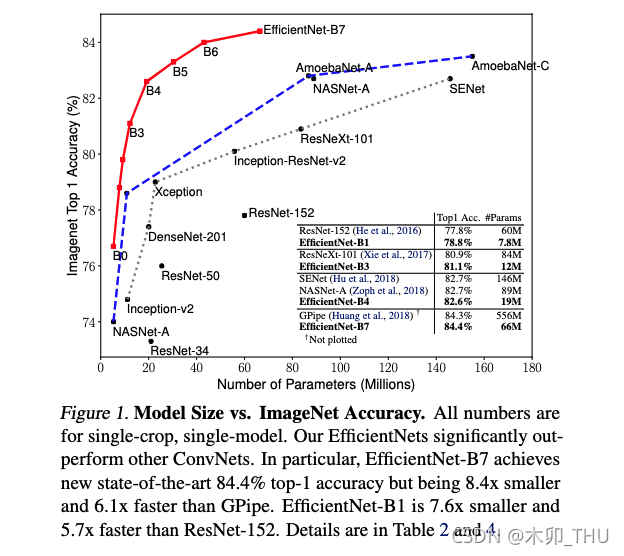
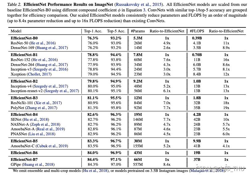
EfficientNetV1 是由Google团队在 2019 年提出的，其原始论文为 EfficientNet: Rethinking Model Scaling for Convolutional Neural Networks。所提出的 EfficientNet-B7 在 Imagenet top-1 上达到了当年最高准确率 84.3%，与之前准确率最高的 GPipe 相比，参数量仅仅为其 1/8.4，推理速度提升了 6.1 倍。本文的核心在于同时探索输入分辨率、网络深度、宽度的影响。下图给出了当时 EfficientNet 以及其他网络的 Top-1 准确率和参数量。我们可以发现，EfficientNet 不仅在参数数量上比很多主流模型小之外，准确率也更高。

请添加图片描述

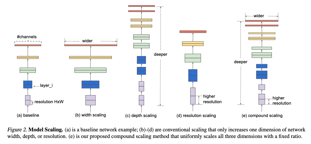
下图给出了模型的结构图。图 a 是传统的卷积神经网络，图 b 在 a 的基础上增大了网络的宽度（即特征矩阵的channel个数），图 c 在 a 的基础上增加了网络的深度（层的个数），图 d 在 a 的基础上增大了输入分辨率（即输入高和宽，这会使得之后所有特征矩阵的高和宽都会相应增加），图 e 即本文考虑的同时增加网络的宽度、深度、以及网络的输入分辨率。

请添加图片描述

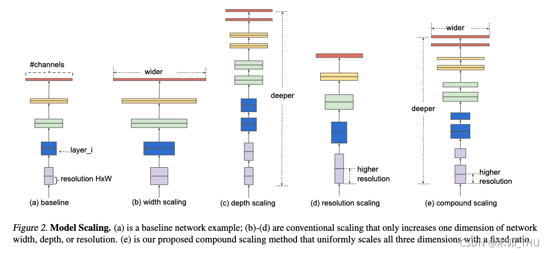
为了提升网络的准确率，一般会考虑增加网络的宽度、深度以及输入图像的分辨率。那么这三个因素是如何影响网络性能的呢？愿论文的部分叙述如下。

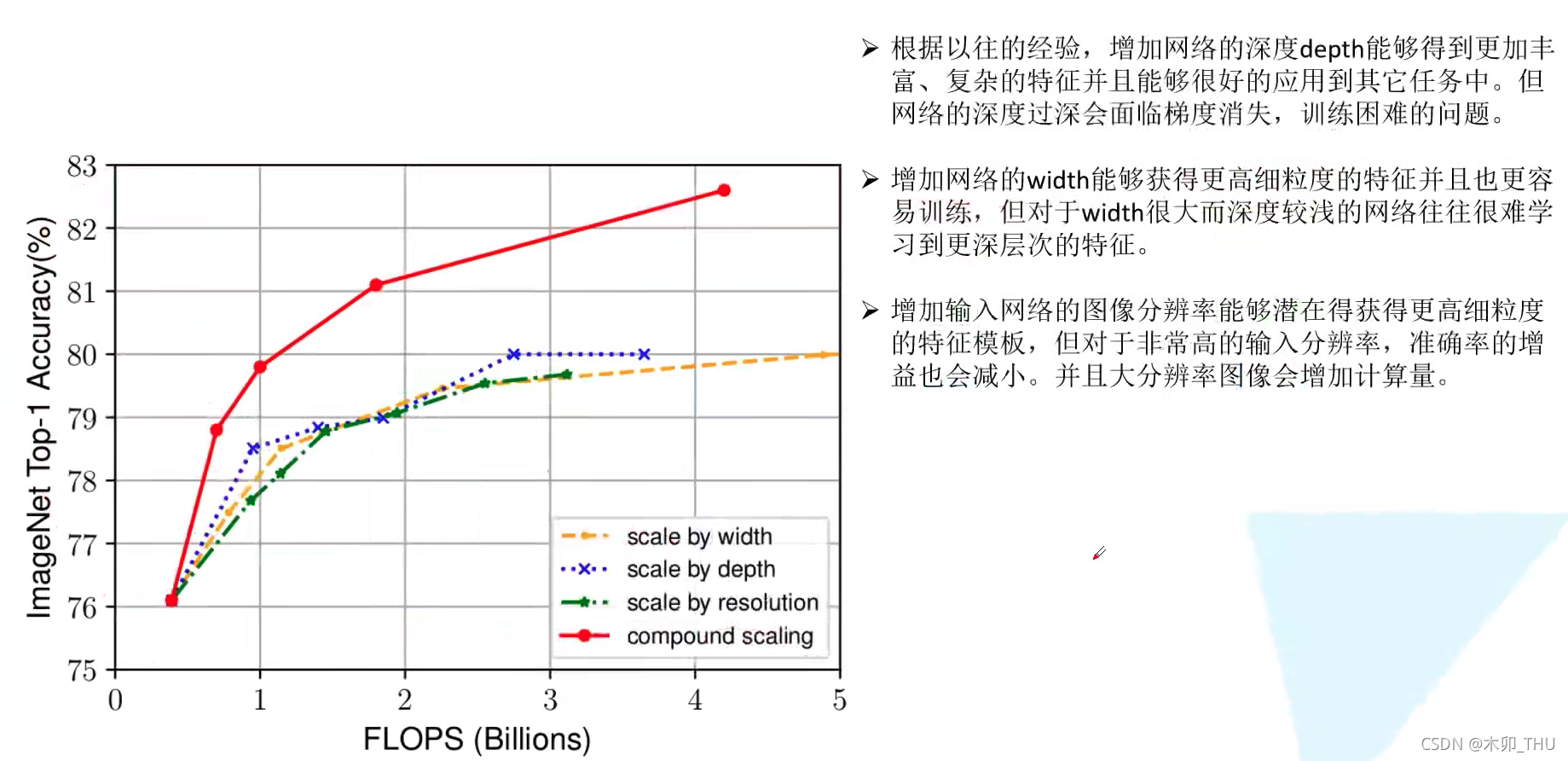
增加网络的深度能够得到更佳丰富、复杂的特征（高级语义），并且能很好的应用到其他任务中去。但是网络的深度过深会面临梯度消失，训练困难等问题。The intuition is that deeper ConvNet can capture richer and more complex features, and generalize well on new tasks. However, deeper networks are also more difficult to train due to the vanishing gradient problem.

增加网络的宽度能够获得更高细粒度的特征，并且也更容易训练。但是对于宽度很大，深度较浅额度网络往往很难学习到更深层次的特征。例如我就只有一个 $\times 3$ 的卷积，但是输出通道为 10000，也没办法得到更为抽象的高级语义。wider networks tend to be able to capture more fine-grained features and are easier to train. However, extremely wide but shallow networks tend to have difficulties in capturing higher level features.

增加输入网络的图像分辨率，能够潜在获得更高细粒度的特征模版，图像分辨率越高能看到的细节就越多，能提升分辨能力。但是对于非常高的输入分辨率，准确率的增益也会减少。且大分辨率图像会增加网络的计算量（注意不是参数量）。With higher resolution input images, ConvNets can potentially capture more fine-grained patterns. but the accuracy gain diminishes for very high resolutions.

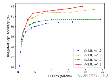
从实验结果可见，分别增加三者在准确率达到 80% 之后就近乎趋于饱和了。我们看，同时调整三者当准确率达到 80% 之后并没有达到饱和，甚至还有更大的提升。这就说明了同时考虑网络的宽度、深度以及输入图像的分辨率，我们可以得到更好的结果。此外我们能看到，当 FLOPs 相同的时候，即理论计算量相同的时候，同时增加这三者，得到的效果也会更好（这其实也就是同时小幅度增加这三个，比单单增加其中一个增加得非常狠要好）。那究竟该如何同时去增加这三者呢？

请添加图片描述

作者还做了实验，即采用不同网络深度 d 和输入分辨率 r 的组合，不断调整网络的宽度 w 得到了如下结果，可以分析出在相同的 FLOPs 的情况下，同时增加网络深度 d 和输入分辨率 r 效果最好。

请添加图片描述

2. 宽度，深度以及分辨率

为什么 ImageNet 训练测试图像要设置为 224？有人说可能是为了和前人对比网络本身的性能要控制变量吧。那第一个跑 ImageNet 的人为什么用 224 呢？可能别人就会说，工程经验。在本文中，EfficientNetV1 使用 NAS（Neural Architecture Search）技术来搜索网络的图像输入分辨率 r，网络的深度 depth 以及 channel 的宽度 width 三个参数的合理化配置。在之前的一些论文中，基本都是通过改变上述3个参数中的一个来提升网络的性能，而这篇论文就是同时来探索这三个参数的影响。

为了探究三者与网络性能之间的关系，作者先在论文中对整个网络的运算进行抽象：
$r)=\bigodot_{i=1 \ldots s} F_{i}^{L_{i}}\left(X_{\left\langle H_{i}, W_{i}, C_{i}\right\rangle}\right)$
其中：

$\bigodot_{i=1 \ldots s}$ 表示连乘运算
$F_i$ 表示一个运算操作，例如后面讲的 MBConv， $F_i^{L_i}$ 表示在 Stage i 中 $F_i$ 运算被重复执行
$X$ 表示输入 Stage 的特征矩阵
$\left\langle H_{i}, W_{i}, C_{i}\right\rangle$ 表示特征矩阵 $X$ 的高度，宽度，以及通道数

随后，为了探究 r，d 和 w 这三个因子对最终准确率的影响，则将 r，d 和 w 加入到公式中，我们可以得到抽象化后的优化问题（在指定资源限制下）：

Our target is to maximize the model accuracy for any given resource constraints, which can be formulated as an optimization problem:

请添加图片描述

其中：

d 用来缩放网络的深度 $\widehat{L}_i$
r 用来缩放特征矩阵的 $\widehat{H}_i, \widehat{W}_i$
w 用来缩放特征矩阵的 $\widehat{C}_i$
target_memory 为内存限制
target_flops 为 FLOPs 限制

需要指出的是：

FLOPs 与d 的关系是：当 d 翻倍，FLOPs 也翻倍。
FLOPs 与w 的关系是：当 w 翻倍，FLOPs 会翻 4 倍，因为卷积层的 FLOPs 约等于 $feature_w \times feature_h \times feature_c \times kernel_w \times kernel_h \times kernel_{number}$ ，假设输入输出特征矩阵的高宽不变，当 width 翻倍，输入特征矩阵的 channels （即 $fearure_c$ ）和输出特征矩阵的 channels（即卷积核的个数， $kernel_{number}$ ）都会翻倍，所以 FLOPs 会翻 4 倍
FLOPs与 r 的关系是：当 r 翻倍，FLOPs 会翻4倍，和上面类似，因为特征矩阵的宽度 $feature_w$ 和特征矩阵的高度 $feature_h$ 都会翻倍，所以 FLOPs 会翻 4 倍

所以总的 FLOPs 倍率可以用近似用 $(\alpha \times \beta^2 \times \gamma^2)^{\phi}$ 来表示，当限制 $\alpha \times \beta^2 \times \gamma^2 \approx 2$ 时，对于任意一个 $\phi$ 而言 FLOPs 相当增加了 $2^{\phi}$ 倍。为此，作者提出了一个混合缩放方法 ( compound scaling method) ，在这个方法中使用了一个混合因子 $\phi$ 去统一的缩放 r，d 和 w 这三个因子，具体的计算公式如下：

请添加图片描述

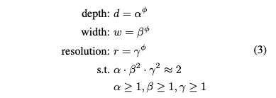
接下来作者在基准网络 EfficientNetB-0（下一小节会讲）上使用 NAS 来搜索 $\alpha, \beta, \gamma$ 这三个参数:

（step1）首先固定 $\phi=1$ ，并基于上面给出的公式 (2) 和 (3) 进行搜索，作者发现对于 EfficientNetB-0 最佳参数为 $\alpha = 1.2 , \beta = 1.1 , \gamma = 1.15$ ，此时 $\alpha \times \beta^2 \times \gamma^2 \approx 1.9203$
（step2）固定 $\alpha = 1.2 , \beta = 1.1 , \gamma = 1.15$ ，在 EfficientNetB-0 的基础上使用不同的 $\phi$ 分别得到 EfficientNetB-1至 EfficientNetB-7。当 $\phi$ = 1 的时候，由公式 (3) 可以得到三者相对于 EfficientNetB-0 的倍率为 $d = 1.2, w = 1.1, r = 1.15$ ，对应的就是 EfficientNetB-2。EfficientNetB-1 则是对应于当 $\phi$ = 0.5 的情况。

原论文指出：对于不同的基准网络搜索出的 $\alpha, \beta, \gamma$ 这三个参数不定相同。作者也说了，如果直接在大模型上去搜索 $\alpha, \beta, \gamma$ 这三个参数可能获得更好的结果，但是在较大的模型中搜索成本太大，所以这篇文章就在比较小的 EfficientNetB-0 模型上进行搜索的。Google 这种大厂都说计算量大，那就是真的大…

Notably, it is possible to achieve even better performance by searching for α, β, γ directly around a large model, but the search cost becomes prohibitively more expensive on larger models. Our method solves this issue by only doing search once on the small baseline network (step 1), and then use the same scaling coefficients for all other models (step 2).

3. EfficientNetV1 网络结构

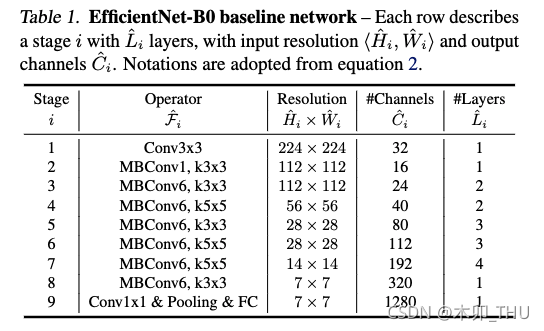
EfficientNet-B0 baseline 网络的结构配置如下图所示，这个网络也是作者通过网络搜索技术得到的。后续讲的 EfficientNet-B1 到 B7 都是在这个网络的基础上进行简单调整的。在 B0 中一共分为 9 个 stage，表中的卷积层后默认都跟有 BN 以及 Swish 激活函数。stage 1 就是一个 $\times 3$ 的卷积层。对于 stage 2 到 stage 8 就是在重复堆叠 MBConv。stage 9 由三部分组成，首先是一个 $\times 1$ 的卷积，然后是平均池化，最后是一个全连接层。表中 Resolution 是每个输入特征矩阵的高度和宽度，Channels 是输出特征矩阵的通道数。Layers 则是将 Operator 重复多少次。stride 参数则是仅针对每个 stage 的第一个 block，之后的 stride 都是 1。

请添加图片描述

紧接着我们来看看 MBConv 模块。论文中说了他和 MobileNetV3 使用的 block 是一样的（那其实单看网络结构没什么contribution，贡献主要在第二节的研究以及推广的model上）。对于主分支而言，首先是一个 $\times 1$ 卷积用于升维，其输出特征矩阵通道是输入 channel 的 n 倍。紧接着通过一个 DW 卷积（这里 DW 卷积的卷积核可能是 $\times 3$ 或者 $\times 5$ ，在上面那个表格中有的，stride 可能等于 1 也可能等于 2）。然后通过一个 SE 模块，使用注意力机制调整特征矩阵。然后再通过 $\times 1$ 卷积进行降维。注意这里只有 BN，没有 swish 激活函数（其实就是对应线性激活函数）。仅当输入 MBConv 结构的特征矩阵与输出的特征矩阵 shape 存在时才有 short-cut 连接，并且在源码中只有使用到 short-cut 连接的 MBConv 模块才有 Dropout 层。同样的，在 stage2 的第一个 MBConv 中，第一个 $\times 1$ 卷积没有升维，所以在实现中没有这个卷积层。

请添加图片描述

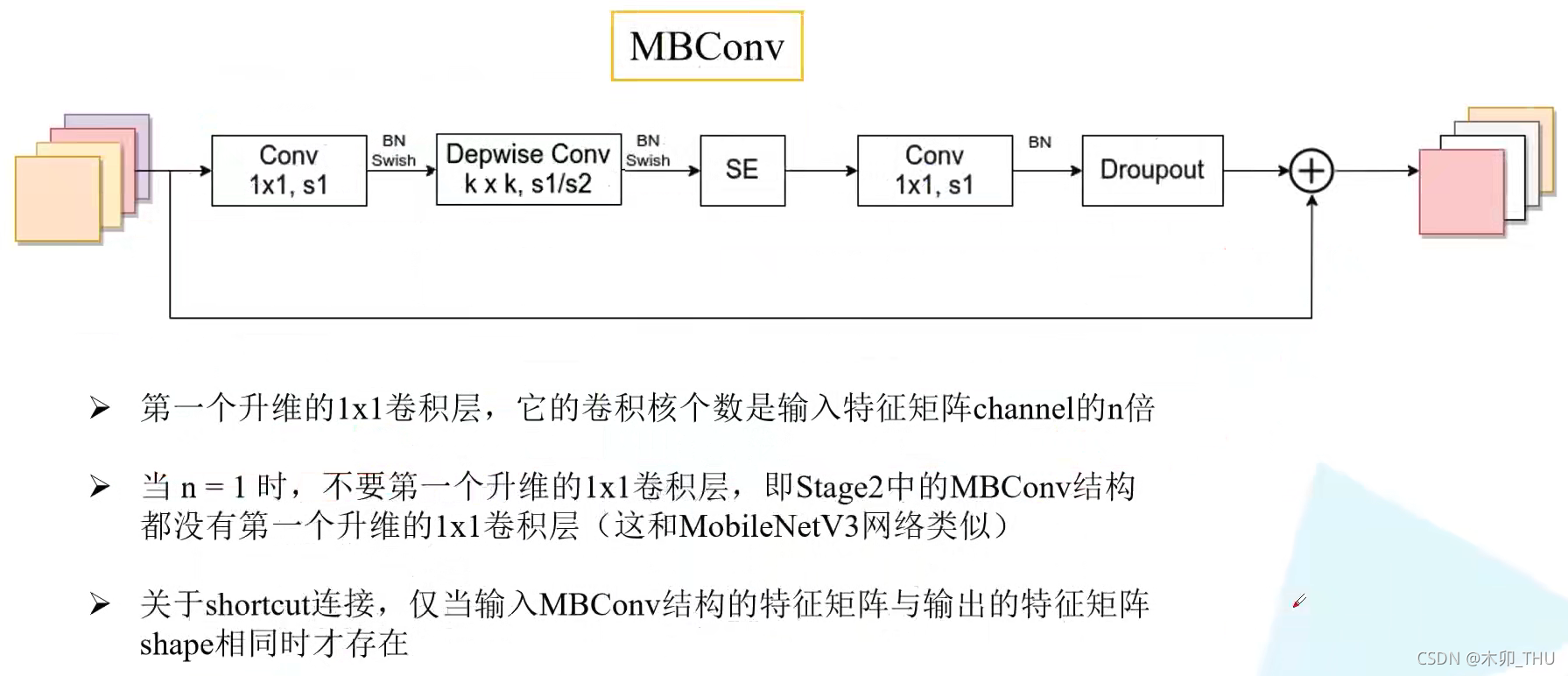
SE 模块在之前 MobileNetV3 的讲解中讲过了，这里再回顾一下。首先对输入矩阵的每个 channel 进行平均池化，然后经过两个全连接层，第一个是 Swish 激活函数，第二个是 Sigmoid 激活函数。第一个全连接层的节点个数等于输入 MBConv 模块的特征矩阵 channel 个数的 1/4（在 MobileNetV3 中是输入 SE 模块的特征矩阵 channel 的 1/4，都是源码中的细节），第二个全连接层的节点个数等于输入 SE 模块的特征矩阵 channel 个数。第二个全连接层的输出其实就是输入 SE 模块的特征矩阵每个 channel 的注意力权重，值越大越重要，越越小越不重要。将权重按通道乘回原特征矩阵就可以了。

请添加图片描述

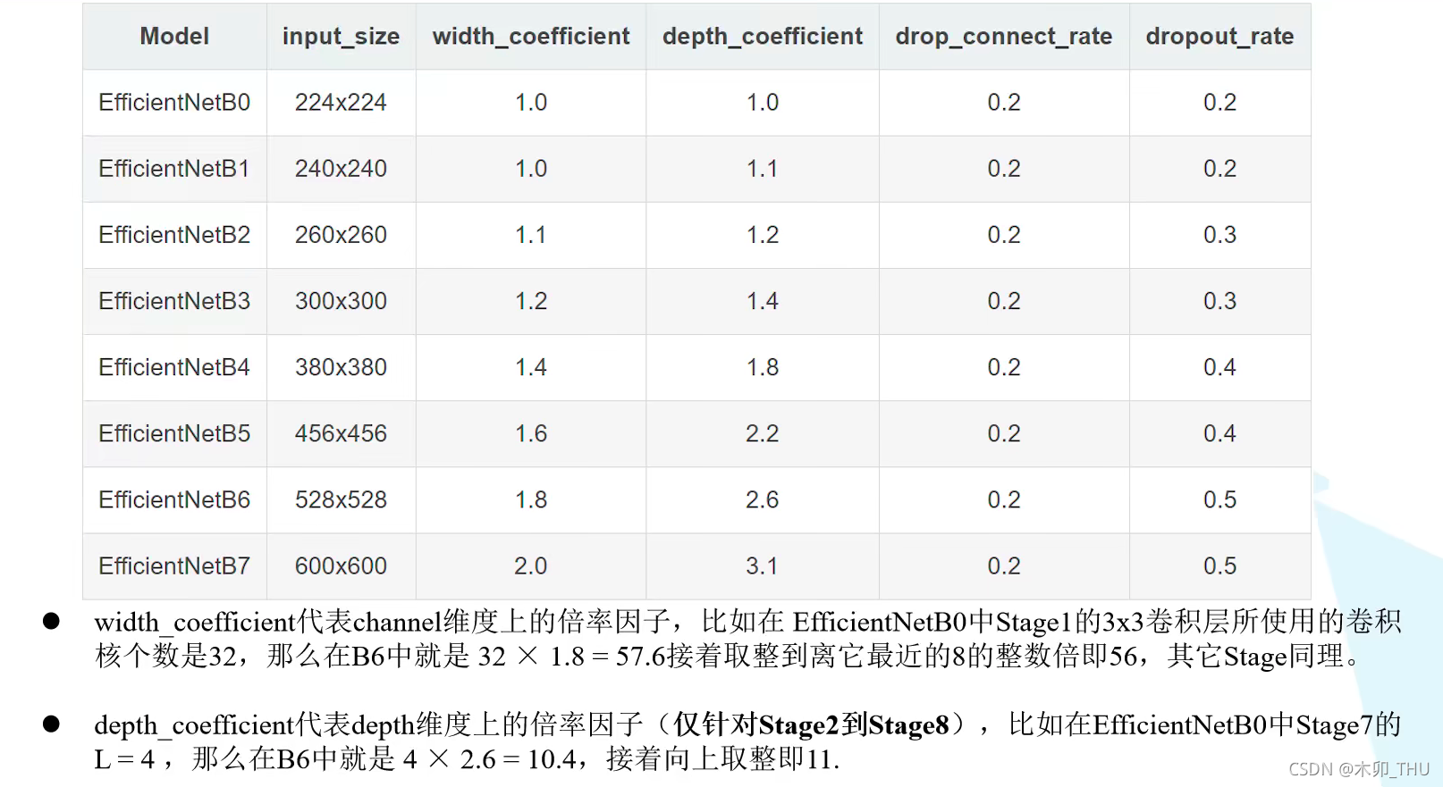
接下来我们看看 EfficientNet-B1 到 B7 是怎么构建出来的。下表分别给出了针对网络宽度，深度的倍率因子，以及对于输入尺寸上的变化。注意，dropout_connect_rate 就是对应上述讲的 MBConv 中的 Dropout 结构的随机失活比率。dropout_rate 对应的是最后一个全连接层前 Dropout 的随机失活比率。

请添加图片描述

性能对比能发现，EfficientNet 就是准确率最高，参数量最小，理论上计算量最低。然而使用中发现，EfficientNet 非常占 GPU 的显存。因为他们输入图像分辨率特别大。速度直接给 FLOPs 就有点耍流氓了，真实运行速度和 FLOPs 不是直接正比的，ShuffleNetV2 就指出，这样做是万万不行滴。

请添加图片描述

4. 代码

EfficientNetV1 实现代码如下所示，代码出处：

import math
import copy
from functools import partial
from collections import OrderedDict
from typing import Optional, Callable

import torch
import torch.nn as nn
from torch import Tensor
from torch.nn import functional as F


def _make_divisible(ch, divisor=8, min_ch=None):
    """
    This function is taken from the original tf repo.
    It ensures that all layers have a channel number that is divisible by 8
    It can be seen here:
    https://github.com/tensorflow/models/blob/master/research/slim/nets/mobilenet/mobilenet.py
    """
    if min_ch is None:
        min_ch = divisor
    new_ch = max(min_ch, int(ch + divisor / 2) // divisor * divisor)
    # Make sure that round down does not go down by more than 10%.
    if new_ch < 0.9 * ch:
        new_ch += divisor
    return new_ch


def drop_path(x, drop_prob: float = 0., training: bool = False):
    """
    Drop paths (Stochastic Depth) per sample (when applied in main path of residual blocks).
    "Deep Networks with Stochastic Depth", https://arxiv.org/pdf/1603.09382.pdf

    This function is taken from the rwightman.
    It can be seen here:
    https://github.com/rwightman/pytorch-image-models/blob/master/timm/models/layers/drop.py#L140
    """
    if drop_prob == 0. or not training:
        return x
    keep_prob = 1 - drop_prob
    shape = (x.shape[0],) + (1,) * (x.ndim - 1)  # work with diff dim tensors, not just 2D ConvNets
    random_tensor = keep_prob + torch.rand(shape, dtype=x.dtype, device=x.device)
    random_tensor.floor_()  # binarize
    output = x.div(keep_prob) * random_tensor
    return output


class DropPath(nn.Module):
    """
    Drop paths (Stochastic Depth) per sample  (when applied in main path of residual blocks).
    "Deep Networks with Stochastic Depth", https://arxiv.org/pdf/1603.09382.pdf
    """
    def __init__(self, drop_prob=None):
        super(DropPath, self).__init__()
        self.drop_prob = drop_prob

    def forward(self, x):
        return drop_path(x, self.drop_prob, self.training)


class ConvBNActivation(nn.Sequential):
    def __init__(self,
                 in_planes: int,
                 out_planes: int,
                 kernel_size: int = 3,
                 stride: int = 1,
                 groups: int = 1,
                 norm_layer: Optional[Callable[..., nn.Module]] = None,
                 activation_layer: Optional[Callable[..., nn.Module]] = None):
        padding = (kernel_size - 1) // 2
        if norm_layer is None:
            norm_layer = nn.BatchNorm2d
        if activation_layer is None:
            activation_layer = nn.SiLU  # alias Swish  (torch>=1.7)

        super(ConvBNActivation, self).__init__(nn.Conv2d(in_channels=in_planes,
                                                         out_channels=out_planes,
                                                         kernel_size=kernel_size,
                                                         stride=stride,
                                                         padding=padding,
                                                         groups=groups,
                                                         bias=False),
                                               norm_layer(out_planes),
                                               activation_layer())


class SqueezeExcitation(nn.Module):
    def __init__(self,
                 input_c: int,   # block input channel
                 expand_c: int,  # block expand channel
                 squeeze_factor: int = 4):
        super(SqueezeExcitation, self).__init__()
        squeeze_c = input_c // squeeze_factor
        self.fc1 = nn.Conv2d(expand_c, squeeze_c, 1)
        self.ac1 = nn.SiLU()  # alias Swish
        self.fc2 = nn.Conv2d(squeeze_c, expand_c, 1)
        self.ac2 = nn.Sigmoid()

    def forward(self, x: Tensor) -> Tensor:
        scale = F.adaptive_avg_pool2d(x, output_size=(1, 1))
        scale = self.fc1(scale)
        scale = self.ac1(scale)
        scale = self.fc2(scale)
        scale = self.ac2(scale)
        return scale * x


class InvertedResidualConfig:
    # kernel_size, in_channel, out_channel, exp_ratio, strides, use_SE, drop_connect_rate
    def __init__(self,
                 kernel: int,          # 3 or 5
                 input_c: int,
                 out_c: int,
                 expanded_ratio: int,  # 1 or 6
                 stride: int,          # 1 or 2
                 use_se: bool,         # True
                 drop_rate: float,
                 index: str,           # 1a, 2a, 2b, ...
                 width_coefficient: float):
        self.input_c = self.adjust_channels(input_c, width_coefficient)
        self.kernel = kernel
        self.expanded_c = self.input_c * expanded_ratio
        self.out_c = self.adjust_channels(out_c, width_coefficient)
        self.use_se = use_se
        self.stride = stride
        self.drop_rate = drop_rate
        self.index = index

    @staticmethod
    def adjust_channels(channels: int, width_coefficient: float):
        return _make_divisible(channels * width_coefficient, 8)


class InvertedResidual(nn.Module):
    def __init__(self,
                 cnf: InvertedResidualConfig,
                 norm_layer: Callable[..., nn.Module]):
        super(InvertedResidual, self).__init__()

        if cnf.stride not in [1, 2]:
            raise ValueError("illegal stride value.")

        self.use_res_connect = (cnf.stride == 1 and cnf.input_c == cnf.out_c)

        layers = OrderedDict()
        activation_layer = nn.SiLU  # alias Swish

        # expand
        if cnf.expanded_c != cnf.input_c:
            layers.update({"expand_conv": ConvBNActivation(cnf.input_c,
                                                           cnf.expanded_c,
                                                           kernel_size=1,
                                                           norm_layer=norm_layer,
                                                           activation_layer=activation_layer)})

        # depthwise
        layers.update({"dwconv": ConvBNActivation(cnf.expanded_c,
                                                  cnf.expanded_c,
                                                  kernel_size=cnf.kernel,
                                                  stride=cnf.stride,
                                                  groups=cnf.expanded_c,
                                                  norm_layer=norm_layer,
                                                  activation_layer=activation_layer)})

        if cnf.use_se:
            layers.update({"se": SqueezeExcitation(cnf.input_c,
                                                   cnf.expanded_c)})

        # project
        layers.update({"project_conv": ConvBNActivation(cnf.expanded_c,
                                                        cnf.out_c,
                                                        kernel_size=1,
                                                        norm_layer=norm_layer,
                                                        activation_layer=nn.Identity)})

        self.block = nn.Sequential(layers)
        self.out_channels = cnf.out_c
        self.is_strided = cnf.stride > 1

        # 只有在使用shortcut连接时才使用dropout层
        if self.use_res_connect and cnf.drop_rate > 0:
            self.dropout = DropPath(cnf.drop_rate)
        else:
            self.dropout = nn.Identity()

    def forward(self, x: Tensor) -> Tensor:
        result = self.block(x)
        result = self.dropout(result)
        if self.use_res_connect:
            result += x

        return result


class EfficientNet(nn.Module):
    def __init__(self,
                 width_coefficient: float,
                 depth_coefficient: float,
                 num_classes: int = 1000,
                 dropout_rate: float = 0.2,
                 drop_connect_rate: float = 0.2,
                 block: Optional[Callable[..., nn.Module]] = None,
                 norm_layer: Optional[Callable[..., nn.Module]] = None
                 ):
        super(EfficientNet, self).__init__()

        # kernel_size, in_channel, out_channel, exp_ratio, strides, use_SE, drop_connect_rate, repeats
        default_cnf = [[3, 32, 16, 1, 1, True, drop_connect_rate, 1],
                       [3, 16, 24, 6, 2, True, drop_connect_rate, 2],
                       [5, 24, 40, 6, 2, True, drop_connect_rate, 2],
                       [3, 40, 80, 6, 2, True, drop_connect_rate, 3],
                       [5, 80, 112, 6, 1, True, drop_connect_rate, 3],
                       [5, 112, 192, 6, 2, True, drop_connect_rate, 4],
                       [3, 192, 320, 6, 1, True, drop_connect_rate, 1]]

        def round_repeats(repeats):
            """Round number of repeats based on depth multiplier."""
            return int(math.ceil(depth_coefficient * repeats))

        if block is None:
            block = InvertedResidual

        if norm_layer is None:
            norm_layer = partial(nn.BatchNorm2d, eps=1e-3, momentum=0.1)

        adjust_channels = partial(InvertedResidualConfig.adjust_channels,
                                  width_coefficient=width_coefficient)

        # build inverted_residual_setting
        bneck_conf = partial(InvertedResidualConfig,
                             width_coefficient=width_coefficient)

        b = 0
        num_blocks = float(sum(round_repeats(i[-1]) for i in default_cnf))
        inverted_residual_setting = []
        for stage, args in enumerate(default_cnf):
            cnf = copy.copy(args)
            for i in range(round_repeats(cnf.pop(-1))):
                if i > 0:
                    # strides equal 1 except first cnf
                    cnf[-3] = 1  # strides
                    cnf[1] = cnf[2]  # input_channel equal output_channel

                cnf[-1] = args[-2] * b / num_blocks  # update dropout ratio
                index = str(stage + 1) + chr(i + 97)  # 1a, 2a, 2b, ...
                inverted_residual_setting.append(bneck_conf(*cnf, index))
                b += 1

        # create layers
        layers = OrderedDict()

        # first conv
        layers.update({"stem_conv": ConvBNActivation(in_planes=3,
                                                     out_planes=adjust_channels(32),
                                                     kernel_size=3,
                                                     stride=2,
                                                     norm_layer=norm_layer)})

        # building inverted residual blocks
        for cnf in inverted_residual_setting:
            layers.update({cnf.index: block(cnf, norm_layer)})

        # build top
        last_conv_input_c = inverted_residual_setting[-1].out_c
        last_conv_output_c = adjust_channels(1280)
        layers.update({"top": ConvBNActivation(in_planes=last_conv_input_c,
                                               out_planes=last_conv_output_c,
                                               kernel_size=1,
                                               norm_layer=norm_layer)})

        self.features = nn.Sequential(layers)
        self.avgpool = nn.AdaptiveAvgPool2d(1)

        classifier = []
        if dropout_rate > 0:
            classifier.append(nn.Dropout(p=dropout_rate, inplace=True))
        classifier.append(nn.Linear(last_conv_output_c, num_classes))
        self.classifier = nn.Sequential(*classifier)

        # initial weights
        for m in self.modules():
            if isinstance(m, nn.Conv2d):
                nn.init.kaiming_normal_(m.weight, mode="fan_out")
                if m.bias is not None:
                    nn.init.zeros_(m.bias)
            elif isinstance(m, nn.BatchNorm2d):
                nn.init.ones_(m.weight)
                nn.init.zeros_(m.bias)
            elif isinstance(m, nn.Linear):
                nn.init.normal_(m.weight, 0, 0.01)
                nn.init.zeros_(m.bias)

    def _forward_impl(self, x: Tensor) -> Tensor:
        x = self.features(x)
        x = self.avgpool(x)
        x = torch.flatten(x, 1)
        x = self.classifier(x)

        return x

    def forward(self, x: Tensor) -> Tensor:
        return self._forward_impl(x)


def efficientnet_b0(num_classes=1000):
    # input image size 224x224
    return EfficientNet(width_coefficient=1.0,
                        depth_coefficient=1.0,
                        dropout_rate=0.2,
                        num_classes=num_classes)


def efficientnet_b1(num_classes=1000):
    # input image size 240x240
    return EfficientNet(width_coefficient=1.0,
                        depth_coefficient=1.1,
                        dropout_rate=0.2,
                        num_classes=num_classes)


def efficientnet_b2(num_classes=1000):
    # input image size 260x260
    return EfficientNet(width_coefficient=1.1,
                        depth_coefficient=1.2,
                        dropout_rate=0.3,
                        num_classes=num_classes)


def efficientnet_b3(num_classes=1000):
    # input image size 300x300
    return EfficientNet(width_coefficient=1.2,
                        depth_coefficient=1.4,
                        dropout_rate=0.3,
                        num_classes=num_classes)


def efficientnet_b4(num_classes=1000):
    # input image size 380x380
    return EfficientNet(width_coefficient=1.4,
                        depth_coefficient=1.8,
                        dropout_rate=0.4,
                        num_classes=num_classes)


def efficientnet_b5(num_classes=1000):
    # input image size 456x456
    return EfficientNet(width_coefficient=1.6,
                        depth_coefficient=2.2,
                        dropout_rate=0.4,
                        num_classes=num_classes)


def efficientnet_b6(num_classes=1000):
    # input image size 528x528
    return EfficientNet(width_coefficient=1.8,
                        depth_coefficient=2.6,
                        dropout_rate=0.5,
                        num_classes=num_classes)


def efficientnet_b7(num_classes=1000):
    # input image size 600x600
    return EfficientNet(width_coefficient=2.0,
                        depth_coefficient=3.1,
                        dropout_rate=0.5,
                        num_classes=num_classes)