机器人学机器学习与控制_机器学习的速度控制_机器学习

机器人学机器学习与控制

介绍(Introduction)

At some point in a machine learning project, you will want to overcome the limitations of your local machine (number of cores, memory, etc.), whether you want to generate a large amount of data to feed deep learning networks or train your algorithms as fast as possible. In this article, we will take you on a journey, sharing the difficulties and the solutions we found, from naive implementation to more advanced techniques, taking advantage of the various computational resources that may be found in the Cloud. We hope this will help you to efficiently manage and improve your productivity for your machine learning projects.

在机器学习项目中的某个时刻，无论您是要生成大量数据来馈入深度学习网络还是要训练算法，您都将要克服本地机器的限制(内核，内存等)。尽可能快地。在本文中，我们将带您走上一段旅程，分享从天真的实现到更先进的技术所遇到的困难和解决方案，并利用云中可能发现的各种计算资源。我们希望这将帮助您有效地管理和提高机器学习项目的生产率。

生成大量数据(例如……很多！) (Generating numerous chunks of data (like… A lot!))

For our experiment, we want to be able to generate a large amount (let’s say 1,000,000) of chunks of data, in a few minutes, to serve as inputs for some Generative Adversarial Networks (GANs). If you have never heard of GANs, you can read my introductory article here [1].

对于我们的实验，我们希望能够在几分钟之内生成大量(比如说1,000,000 )数据块，以作为某些生成对抗网络(GAN)的输入。如果您从未听说过GAN，可以在这里阅读我的介绍性文章[1]。

The chunks we are talking about will be cubes of dimension n=100 (i.e. 1,000,000 of data points). This specific number of 1 megavoxels (data points for volumes) has been chosen to match the current state of the art of generating fake faces, that can be seen on the website thispersondoesnotexist.com. The technique used there is called StyleGAN2 [2] (a variant of GANs), where generated images are of size 1024 x 1024, thus on the order of magnitude of 1 megapixels.

我们正在讨论的块将是尺寸为n = 100(即1,000,000个数据点)的多维数据集。已选择此特定数量的1兆体素(体积的数据点)，以匹配生成假脸的当前技术水平，这可以在thispersondoesnotexist.com网站上看到。那里使用的技术称为StyleGAN2 [2](GAN的变体)，其中生成的图像大小为1024 X 1024，因此约为1兆像素。

In order to reflect some data preparation from the real world, additional constraints will apply to build our cubes. They will be derived from dataframes and will be the result of stacking numpy arrays. For the sake of simplicity, those dataframes will have random values.

为了反映来自现实世界的一些数据准备，附加的约束将应用于构建我们的多维数据集。它们将从数据帧派生，并且是堆叠numpy数组的结果。为了简单起见，这些数据帧将具有随机值。

The objective here is to create cubes as fast as possible !

这里的目标是尽可能快地创建多维数据集！

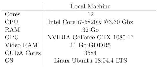
The first steps will be done on our local machine, which specs are described in Table 1. As you can see, this is already a pretty nice setup.

第一步将在我们的本地计算机上完成，其规格在表1中进行了描述。您可以看到，这已经是非常不错的设置。

Image for post — Table 1: Specifications of our local machine.

输入数据 (Input Data)

We first generate 100 dataframes of size 1000 x 1000, containing random floats (rounded to 10 decimals), thanks to the numpy.random.rand function. The dataframes are then saved to disk using the pandas.DataFrame.to_csv function. Each csv file is about 13 Mo.

我们首先生成大小为1000的100个数据帧 X 1000，由于numpy.random.rand函数，包含随机浮点数(四舍五入到10位小数)。然后使用pandas.DataFrame.to_csv函数将数据帧保存到磁盘。每个csv文件约为13Mo。

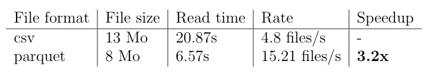
For each cube, we will have to use all the dataframes to extract a random subset from them. Using the pandas.read_csv function, it takes 20.87s to read all the dataframes, hence 4.79 files/s. This is very slow. For the record, if we wanted to build 1,000,000 cubes, at this pace, it would take more than 240 days !

对于每个多维数据集，我们将不得不使用所有数据帧从中提取随机子集。使用pandas.read_csv函数，读取所有数据帧需要20.87秒，因此需要4.79个文件/秒。这很慢。记录下来，如果我们要以这种速度建造1,000,000个多维数据集，则将需要240天以上的时间！

Instead of using the csv format, let’s consider the parquet file format to save our dataframes. Using the fastparquet engine [3], each saved parquet file is now only 8 Mo. If you want to learn more about the parquet file format, you can check the official website here [4]. This time, reading all the 100 dataframes only takes 6.57s (or 15.21 files/s)! This represents a 3.2x speedup. Those first results are gathered in Table 2.

让我们考虑使用实木复合地板文件格式来保存数据帧，而不是使用csv格式。现在，使用fastparquet引擎[3]，每个保存的实木复合地板文件只有8Mo 。如果您想了解有关实木复合地板文件格式的更多信息，可以在此处查看官方网站[4]。这次，读取所有100个数据帧仅需6.57 s (或15.21个文件/ s)！这表示加速了3.2倍。这些最初的结果汇总在表2中。

建立我们的第一个立方体 (Building Our First Cubes)

Using some constraints, the following steps will apply to build one cube:

使用一些约束，以下步骤将应用于构建一个多维数据集：

For each dataframe, we extract a sub-dataframe containing the first 100 rows and 100 random columns,
对于每个数据框，我们提取一个子数据框，其中包含前100行和100个随机列，
Each sub-dataframe is then converted to a numpy array of dimension 100 x 100,
然后将每个子数据帧转换为尺寸为100 x 100的numpy数组，
The numpy arrays are stacked to create one cube.
将numpy数组堆叠以创建一个多维数据集。

# CREATING THE CUBES FROM FILES (READ IN A LOOP)import numpy as np
import pandas as pdncubes = 100
dim = 100for n in range(ncubes):
    cube = np.zeros(shape=(dim, dim, dim))
    # 'files_list' is the list of the parquet file paths
    for i, f in enumerate(files_list):
        df = pd.read_parquet(f)
        df = df.head(dim)
        rnd_cols = random.sample(range(1, df.shape[1]), dim)
        df = df.iloc[:, rnd_cols]
        layer = df.to_numpy()
        cube[i, :, :] = layer

The total time to get a batch of 100 cubes is about 661s (almost 11 minutes), hence a rate of 0.15 cubes/s.

一批100立方的总时间约为661s(将近11分钟)，因此速率为0.15立方/秒。

I’m sure you already spotted the mistake here. Indeed, for each cube, we read the same 100 parquet files every time! In practice, you surely don’t want to loop over those files. The next improvement regarding the data structure is going to fix this.

我确定您已经在这里发现了错误。实际上，对于每个多维数据集，我们每次都读取相同的100个实木复合地板文件！实际上，您当然不希望遍历这些文件。关于数据结构的下一个改进将解决此问题。

提高速度-步骤1：数据结构 (Improving Speed — Step 1: The Data Structure)

Since we don’t want to read the parquet files inside the loop for each cube, it could be a good idea to perform this task only once and upfront. So, we can build a dictionary df_dict, having files names as keys and dataframes as values. This operation is pretty fast and the dictionary is built in 7.33s only.

由于我们不想在每个多维数据集的循环内读取镶木地板文件，因此最好一次只执行一次此任务。因此，我们可以构建字典df_dict ，将文件名作为键，将数据帧作为值。此操作非常快，并且字典仅在7.33s内构建。

Now, we are going to write a function to create a cube, taking advantage of that dictionary already having dataframes read and stored as its own values.

现在，我们将编写一个函数来创建一个多维数据集，利用该字典已经读取和存储了自己的值的数据帧。

# FUNCTION CREATING A CUBE FROM A DICTIONARY OF DATAFRAMESdef create_cube(dimc, dict_df):
    cube = np.zeros(shape=(dimc, dimc, dimc))
    for i, df in enumerate(dict_df.values()):
        df = df.head(dimc)
        rnd_cols = random.sample(range(1, df.shape[1]), dimc)
        df = df.iloc[:, rnd_cols]
        layer = df.to_numpy()
        cube[i, :, :] = layer
    return cube

This time, creating 100 cubes only took 6.61s for a rate of 15.13 cubes/s. This represents a 100x speedup compared to the previous version not using the dictionary of dataframes. Creating our batch of 1,000,000 cubes would now only take nearly 20 hours instead of the initial 240 days.

这次，创建100个多维数据集仅花费了6.61秒，速率为15.13多维数据集/秒。与不使用数据帧字典的先前版本相比，这代表了100倍的加速。现在，创建我们的1,000,000多维数据集批次仅需将近20小时，而不是最初的240天。

Now, we still use dataframes to build our cubes, maybe it’s time to go full NumPy to increase our speed.

现在，我们仍然使用数据框构建多维数据集，也许是时候使用完整的NumPy来提高速度了。

提高速度-步骤2：NumPy摇滚！ (Improving Speed — Step 2: NumPy Rocks!)

The previous idea of using a dictionary of dataframes was interesting but may be improved by building, from the very beginning, a numpy.ndarray derived from the parquet files, from which we will sub-sample along the columns to create our cubes. Let’s first create this big boy:

以前使用数据帧字典的想法很有趣，但是可以通过从一开始构建从numpy.ndarray文件派生的numpy.ndarray加以改进，然后我们将沿着列对它们进行子采样以创建多维数据集。首先创建一个大男孩：

# CREATING THE RAW DATA (NUMPY FORMAT)arr_data = np.zeros(shape=(100, 1000, 1000))
# 'files_list' is the list of the parquet file paths
for i, j in enumerate(files_list):
    df = pd.read_parquet(j)
    layer = df.to_numpy()
    arr_data[i, :, :] = layer

Then, we have to modify our create_cube function accordingly and implement a full vectorization:

然后，我们必须相应地修改create_cube函数并实现完整的矢量化：

# FUNCTION CREATING A CUBE FROM RAW DATA (FULL NUMPY VERSION)def create_cube_np(dimc):
    rnd_cols = random.sample(range(1, 1000), dimc)
    # First 100 rows, 100 random columns (vectorization)
    cube = arr_data[:, :100, rnd_cols]
    return cube

Using this new version, we are able to create 100 cubes in just 1.31s, hence a nice rate of 76.26 cubes/s.

使用这个新版本，我们能够在1.31s内创建100个多维数据集，因此速率为76.26 cubes / s 。

Now, we can move on to the next step to go even faster. You guessed it, time for parallelization!

现在，我们可以继续下一步以更快地进行操作。您猜对了，该进行并行化了！

提高速度-步骤3：并行化 (Improving Speed — Step 3: Parallelization)

There are several ways to perform parallelization in Python [5][6]. Here, we will use the native multiprocessing Python package along with the imap_unordered function to perform asynchronous jobs. We plan to take advantage of the 12 cores from our local machine.

在 Python [5] [6]中有几种执行并行化的方法。在这里，我们将使用本机multiprocessing Python包以及imap_unordered函数来执行异步作业。我们计划利用本地计算机的12个内核。

# PARALLELIZATIONfrom multiprocessing import ThreadPoolproc = 12  # Number of workers
ncubes = 100
dim = 100def work(none=None):
    return create_cube_np(dim)with ThreadPool(processes=proc) as pool:
    cubes = pool.imap_unordered(work, (None for i in range(ncubes)))
    for n in range(ncubes):
        c = next(cubes)  # Cube is retrieved here

The ThreadPool package is imported here (instead of the usual Pool package) because we want to ensure the following:

ThreadPool软件包(而不是通常的Pool软件包)被导入此处，因为我们要确保以下几点：

Stay inside the same process,
保持相同的过程，
Avoid transfer data between processes,
避免在流程之间传输数据，
Getting around the Python Global Interpreter Lock (GIL) by using numpy-only operations (most of numpy calculations are unaffected by the GIL).
使用仅numpy的操作来解决Python全局解释器锁(GIL)(大多数numpy计算不受GIL的影响)。

You can learn more about the difference between multiprocessing and multithreading in Python in this nice blog post [7].

您可以在这篇不错的博客文章[7]中了解有关Python中多处理和多线程之间的区别的更多信息。

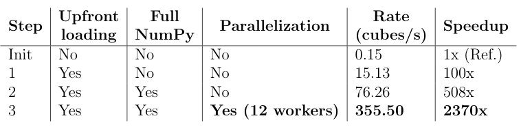
Using this multithreading approach, we only need 0.28s to create one batch of 100 cubes. We reach a very good rate of 355.50 cubes/s, hence a 2370x speedup compared to the very first version (Table 3). Regarding our 1,000,000 cubes, the generation time has dropped under an hour.

使用这种多线程方法，我们只需要0.28s即可创建一批100个多维数据集。我们达到了355.50立方/秒的非常高的速率，因此与第一个版本(表3 )相比，提速了2370倍。对于我们的1,000,000个立方体，生成时间已减少了不到一个小时。

Now, it’s time to fly by using virtual machine instances in the Cloud!

现在，是时候通过在云中使用虚拟机实例飞！

提高速度-步骤4：云端 (Improving Speed — Step 4: The Cloud)

If we talk about Machine Learning as a Service (MLaaS), the top 4 cloud solutions are: Microsoft Azure, Amazon AWS, IBM Watson and Google Cloud Platform (GCP). In this study, we chose GCP but any other provider would do the job. You can select or customize your own configuration among a lot of different virtual machine instances, where you will be able to execute your code inside a Notebook.

如果我们谈论机器学习即服务( MLaaS )，则排名前四的云解决方案是：Microsoft Azure，Amazon AWS，IBM Watson和Google Cloud Platform(GCP)。在本研究中，我们选择了GCP，但其他任何提供者都可以胜任。您可以在许多不同的虚拟机实例中选择或定制自己的配置，从而可以在Notebook中执行代码。

The first question you want to ask yourself is the following one:

您要问自己的第一个问题是以下问题：

“What kind of instance do I want to create that matches my computation needs ?”

“我想创建什么样的实例来满足我的计算需求？”

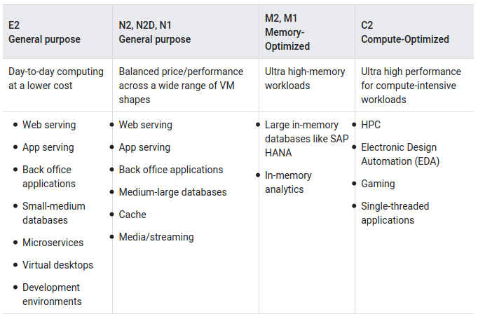
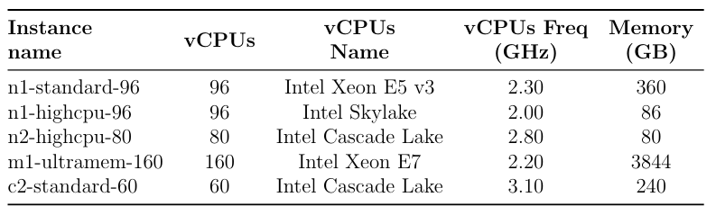
Basically, you can find three types of machines: general purpose, memory-optimized or compute-optimized (Table 4).

基本上，您可以找到三种类型的计算机：通用计算机，内存优化计算机或计算优化计算机(表4 )。

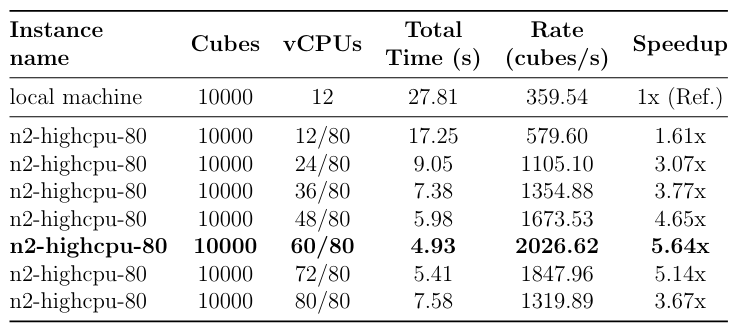
To compute the numpy.ndarray from Step 2, parquet files are first stored into a bucket in the Cloud. Then, several tests are conducted on different VM instances (Table 5), keeping the same multithreading code as in Step 3, and progressively increasing the number of vCPUs (workers). An example of results for one virtual machine is presented in Table 6.

计算numpy 。 步骤2中的ndarray ，首先将实木复合地板文件存储到Cloud中的存储桶中。然后，在不同的VM实例上进行了几次测试(表5 )，保持与步骤3中相同的多线程代码，并逐渐增加vCPU(工作人员)的数量。表6中显示了一个虚拟机的结果示例。

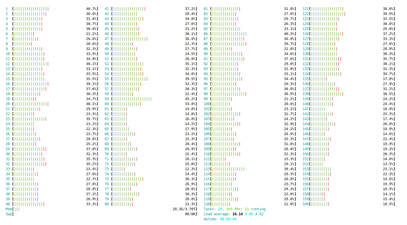
In a terminal connected to your virtual machine, you can also visualize the activity of your vCPUs, using the htop linux command (Figure 1).

在连接到虚拟机的终端中，您还可以使用htop linux命令可视化vCPU的活动(图1 )。

结论 (Conclusion)

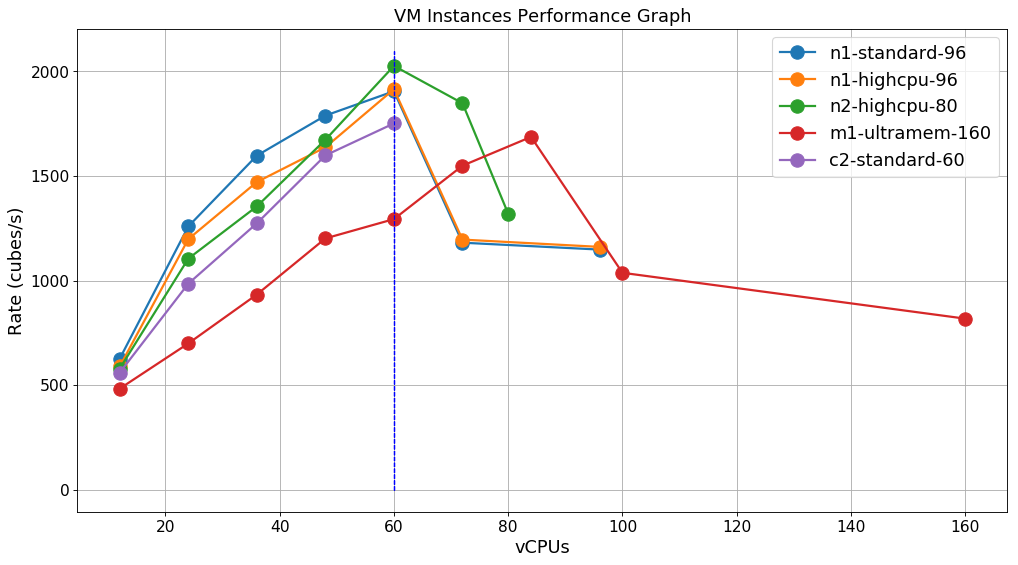
Looking at Figure 2, except for the m1-ultramem-160 instance (which is the most expensive), all the other instances perform pretty well, but follow the same pattern. The rate is increasing almost linearly with the number of workers and reaches a peak at 60 vCPUs. Beyond that limit, the rate drops drastically, most probably because of the overhead of the multithreading.

从图2可以看出，除了m1-ultramem-160实例(这是最昂贵的)之外，所有其他实例的性能都很好，但是遵循相同的模式。该速率几乎随着工人数量呈线性增长，并在60个vCPU处达到峰值。超过该限制，速率急剧下降，最有可能是由于多线程的开销。

Among our selection, the winner is the n2-highcpu-80 instance (the second cheapest), reaching a rate of 2026.62 cubes/s, almost 2 billion data points per second. At this pace, we can generate 1,000,000 cubes in only 8 minutes.

在我们的选择中，获胜者是n2-highcpu-80实例(第二便宜的实例)，达到2026.62立方/秒的速度，每秒近20亿个数据点。以这种速度，我们仅用8分钟就可以生成1,000,000个多维数据集。

Our initial objective was successfully achieved !

我们的最初目标已成功实现！

This whole experiment demonstrates that not only code matters but hardware too. We began with a rate of 0.15 cubes/s on our local machine to reach a very quick rate of 2027 cubes/s, using the Cloud. This is more than a 13,500x speedup !

整个实验表明，不仅代码很重要，硬件也很重要。我们使用Cloud在本地计算机上以0.15立方/秒的速率开始，很快达到2027立方/秒的速率。这不仅仅是13,500倍的加速！

And this is just the beginning… We can level up by using more advanced technologies and infrastructures. This would be for Episode 2.

而这仅仅是个开始......我们可以用更先进的技术和基础设施升级。这将是第2集。