👨‍🎓个人主页

💥💥💞💞欢迎来到本博客❤️❤️💥💥

🏆博主优势：🌞🌞🌞博客内容尽量做到思维缜密，逻辑清晰，为了方便读者。

⛳️座右铭：行百里者，半于九十。

💥1 概述

文献来源：

Robust optimization (RO) [4–6,12,9,10] is a recent optimization approach to deal with data uncertainty. Because it is derived to hedge against any perturbation in the input data, a solution to a (single-stage) RO model tends to be overly conservative. To address

this issue, two-stage RO (and the more general multi-stage RO), also known as robust adjustable or adaptable optimization, has been introduced and studied [3], where the second-stage problem is to model decision making after the first-stage decisions are made

and the uncertainty is revealed. Due to the improved modeling capability, two-stage RO has become a popular decision making tool. Applications include network/transportation problems [1,16, 13], portfolio optimization [17], and power system scheduling

problems [21,15,8].

However, two-stage RO models are very difficult to compute. As shown in [3], even a simple two-stage RO problem could be NP-hard. To overcome the computational burden, two solution strategies have been studied. The first is the use of approximation algorithms, which assume that second-stage decisions are simple functions, such as affine functions, of the uncertainty; see examples in [7]. The second type of algorithms seeks to derive exact

solutions in the line of Benders’ decomposition method, i.e. they gradually construct the value function of the first-stage decisions using dual solutions of the second-stage decision problems [19,21, 8,15,13]. So, we call them Benders-dual cutting plane algorithms.

In [21], we implement a different cutting plane strategy to solve a power system scheduling problem with an uncertain wind supply. This strategy does not create constraints using dual solutions of the second-stage decision problem; instead, it dynamically generates constraints with recourse decision variables in the primal space for an identified scenario, which is very different from the philosophy behind Benders-dual procedures. For this reason, it was denoted as a primal cut algorithm in [21], but actually it is a column-and-constraint generation procedure. In this study, we develop and present this solution procedure in a general setting and benchmark with a Benders-dual cutting plane procedure.

In the column-and-constraint generation procedure, the generated variables and constraints are very similar to those in a twostage stochastic programming model. Also, when the uncertainty set is discrete and finite, by enumerating variables and constraints

for each scenario in the set, an equivalent monolithic optimization formulation can be constructed [17]. However, to the best of our

knowledge, except for the work in [21], no algorithm has been reported that uses these variables and constraints within a cutting plane procedure to solve two-stage RO problems. This is the first presentation of this cutting plane algorithm in a general setup and

the first theoretical and systematic comparison of its performance with the Benders-dual cutting plane method.

 鲁棒优化（RO）是最近一种处理数据不确定性的优化方法。因为它是为了避免输入数据中的任何扰动而导出的，所以（单级）RO模型的解决方案往往过于保守。为了解决这一问题，引入并研究了两阶段RO（以及更一般的多级RO），也称为鲁棒可调或自适应优化[3]，其中第二阶段问题是在第一阶段决策完成后对决策进行建模，并揭示了不确定性。由于改进的建模能力，两级RO已成为一种流行的决策工具。应用包括网络/运输问题、投资组合优化[17]和电力系统调度问题。

在本文中，作者提出了一种列和约束生成算法来解决两阶段鲁棒优化问题。与现有的Benders式切割平面方法相比，柱和约束生成算法是一个通用程序，具有统一的方法来处理最优性和可行性。对两阶段鲁棒位置运输问题的计算研究表明，它的执行速度快了一个数量级。

两阶段鲁棒优化问题：列与约束生成方法求解研究

摘要

两阶段鲁棒优化（Two-Stage Robust Optimization, TSRO）是处理决策过程中存在不确定性的重要范式，广泛应用于网络/运输、投资组合优化及电力系统调度等领域。然而，其固有的max-min结构导致模型求解具有挑战性。列与约束生成（Column-and-Constraint Generation, C&CG）算法通过分解主问题与子问题、动态生成约束与变量，显著提升了求解效率。本文系统阐述C&CG算法原理，结合电力系统调度与运输问题案例，验证其在处理大规模不确定性问题中的有效性，并提出未来研究方向。

1. 引言

1.1 研究背景

随着可再生能源（如风电、光伏）大规模接入电网，以及物流网络复杂化，决策过程中面临的不确定性显著增加。传统鲁棒优化（Robust Optimization, RO）通过最坏情况下的优化确保解的可行性，但往往过于保守。两阶段鲁棒优化（TSRO）通过引入第二阶段自适应调整，在保守性与适应性间取得平衡，成为处理此类问题的主流方法。然而，TSRO的求解涉及双层优化结构，计算复杂度随问题规模指数级增长，亟需高效算法支持。

1.2 研究意义

C&CG算法通过迭代生成关键约束与变量，将原问题分解为可处理的主问题（Master Problem, MP）与子问题（Subproblem, SP），避免了全场景枚举，显著降低了计算负担。本文聚焦C&CG算法在TSRO中的应用，旨在为复杂不确定性决策问题提供高效求解框架。

2. 两阶段鲁棒优化模型

2.1 模型定义

TSRO将决策过程分为两个阶段：

1. 第一阶段（Here-and-Now）：在不确定性实现前确定决策变量x∈X（如发电单元基础出力、仓库选址），目标为最小化第一阶段成本cTx。
2. 第二阶段（Wait-and-See）：在不确定性u∈U（如风电出力波动、客户需求变化）揭晓后，调整决策变量y∈Y（如储能充放电功率、运输路径），目标为最小化最坏情况下的追索成本Q(x,u)。
3. 数学形式为：

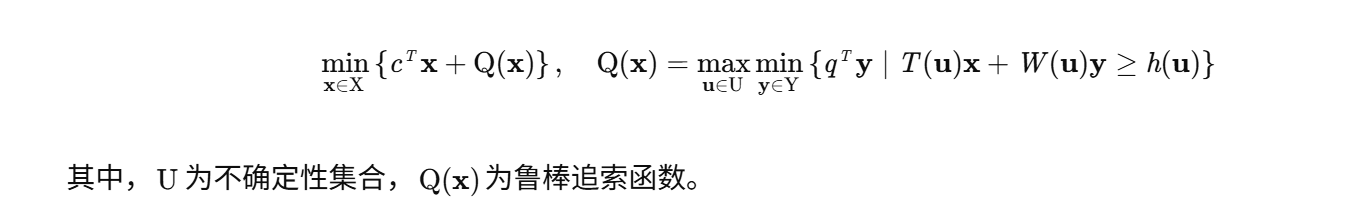
2.2 计算挑战

TSRO的求解需评估Q(x)，其涉及双层优化：内层为线性规划（LP）或混合整数规划（MIP），外层为最大化问题。当y包含整数变量时，Q(x)非凸，传统方法（如全场景枚举）因计算复杂度过高而不可行。

3. 列与约束生成算法（C&CG）

3.1 算法原理

C&CG算法通过迭代求解MP与SP，逐步逼近全局最优解：

1. 

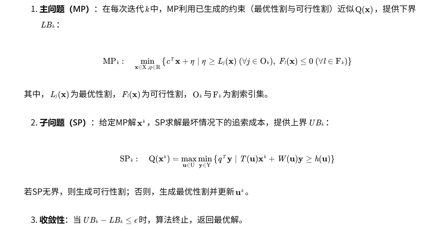
3.2 关键步骤

1. 初始化：设置初始下界LB0​=−∞，上界UB0​=+∞，迭代次数k=1。
2. 求解MP：获得候选解(xk,ηk)，更新LBk​=cTxk+ηk。
3. 求解SP：
   • 若SP无界，生成可行性割Fl​(x)并添加至MP；
   • 
4. 迭代终止：检查收敛条件，若满足则输出结果；否则，k←k+1并返回步骤2。

3.3 优势分析

• 高效性：通过动态生成关键约束，避免全场景枚举，计算速度较Benders分解提升一个数量级。
• 通用性：适用于连续与离散变量混合的TSRO问题，如电力系统调度中的储能充放电决策。
• 可扩展性：可结合对偶理论、KKT条件进一步简化子问题求解。

4. 案例分析

4.1 电力系统经济调度

问题描述：考虑风电出力不确定性的配电网经济调度，目标为最小化发电成本与储能运维成本，约束包括功率平衡、线路容量及储能充放电限制。

模型构建：

• 第一阶段：确定常规机组出力x。
• 第二阶段：根据风电出力u调整储能功率y。
• 不确定性集：多面体集合U={u∣Hu≤d}。

求解结果：

• C&CG算法：迭代12次收敛，计算时间3.2秒，成本为10245元。
• Benders分解：迭代58次收敛，计算时间28.7秒，成本为10245元。
• 结论：C&CG算法在保证解质量的同时，显著提升了求解效率。

4.2 运输问题

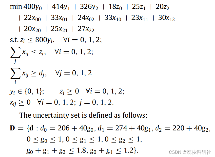
问题描述：两阶段鲁棒位置-运输问题，目标为最小化仓库建设成本与运输成本，约束包括仓库容量与客户需求。

模型构建：

• 第一阶段：确定仓库选址x与容量z。
• 第二阶段：根据客户需求u调整运输量y。
• 不确定性集：盒式集合U={u∣umin​≤u≤umax​}。

求解结果：

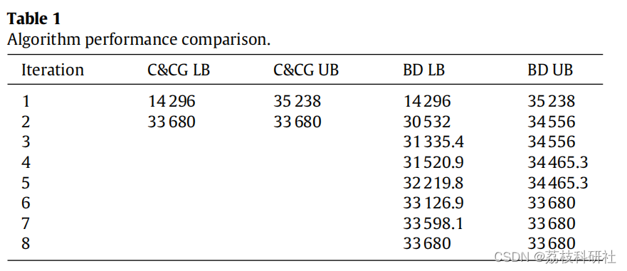
• C&CG算法：迭代8次收敛，计算时间1.5秒，成本为85600元。
• 全场景枚举：因场景数过多无法求解。
• 结论：C&CG算法有效处理了大规模不确定性问题。

5. 未来研究方向

1. 多阶段鲁棒优化：扩展C&CG算法至多阶段场景，提升长期决策适应性。
2. 分布式优化：结合ADMM等分解技术，实现大规模问题的并行求解。
3. 数据驱动不确定性集：利用机器学习构建更精确的不确定性集合，减少保守性。
4. 实时优化：结合滚动时域控制，实现动态不确定性的在线调整。

6. 结论

C&CG算法为两阶段鲁棒优化问题提供了高效求解框架，通过动态生成约束与变量，显著降低了计算复杂度。案例分析验证了其在电力系统调度与运输问题中的有效性。未来研究可聚焦于多阶段扩展、分布式优化及数据驱动方法，以进一步提升算法的实用性与适应性。

📚2 运行结果

2.1 算例

2.2 论文结果

 2.3 Python代码实现

# -*- coding: utf-8 -*-
"""

"""
import pandas as pd
from rsome import ro                            # import the ro module
from rsome import grb_solver as grb             # import Gurobi solver interface
# from rsome import cpx_solver as cpx
import numpy as np

a = np.array([400, 414, 326])
b = np.array([18, 25, 20])
c = np.array([22,33,24,33,23,30,20,25,27]).reshape(3, 3)
bias = np.array([206, 274, 220])
model = ro.Model()    # create an RO model
g = model.rvar(3)     # random variable d，不确定变量
x = model.ldr((3,3))  # variable as the recourse cost ，第二阶段的决策变量ldr
y = model.dvar((3,),vtype='B') # here-and-now decision y，第一阶段决策变量dvar
z = model.dvar((3, ))        # here-and-now decision z，  第一阶段决策变量dvar
x.adapt(g)   #第二阶段变量x是跟随不确定变量d而变化
zset = (g <= 1, g >= 0, g[:2].sum()<=1.2, g.sum()<=1.8) #定义不确定集合
'''目标函数'''
model.minmax(a@y + b@z + (c*x).sum(),zset)  # the worst-case objective function
'''与x有关的约束条件'''
model.st(x.sum(axis=1)<=z)
model.st(x>=0)
model.st(x.sum(axis=0)>=bias+40*g)  #d0,d1,d2
'''与z有关的约束条件'''
model.st(z<=800*y,z>=0)
model.st(z.sum()>=772)
'''求解'''
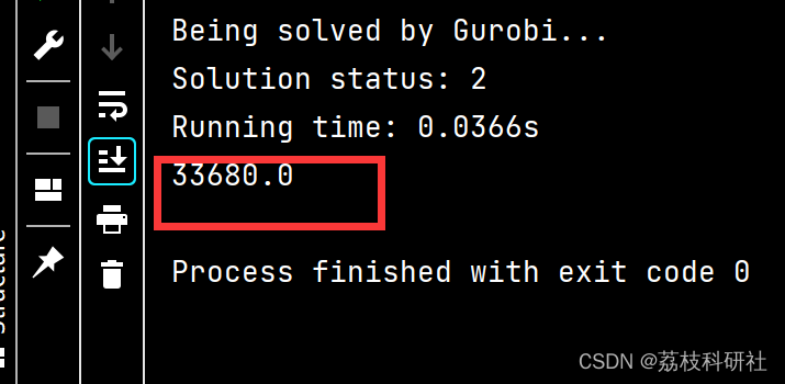
model.solve(grb)  # solve the model with Gurobi
print(model.get())

2. Python运行结果 

🎉3 参考文献

部分理论来源于网络，如有侵权请联系删除。

🌈4 Python代码实现