工业级视觉缺陷检测：利用 CNN 进行高精度无损筛查与分类实践

sequenceDiagram
    participant Client as 客户端
    participant API as 网关层
    participant Service as 业务服务
    participant DB as 数据库
    
    Client->>API: 请求数据
    API->>Service: 处理业务逻辑
    Service->>DB: 查询数据
    DB-->>Service: 返回结果
    Service-->>API: 返回处理结果
    API-->>Client: 返回响应

一、引言

在"中国制造2025"和工业4.0的浪潮下，传统制造业正经历着前所未有的智能化转型。其中，产品质量检测作为制造业最核心的环节之一，长期以来依赖人工目视检查。人工检测不仅效率低下、成本高昂，更严重的问题是检测标准不稳定——不同质检员的标准存在差异，同一位质检员在不同疲劳程度下的判断也不一致。

据制造业行业统计，传统人工目检的缺陷漏检率通常在10%-30%之间，而误检率可能高达20%。对于高价值产品（如半导体芯片、精密光学元件、航空航天零部件），一旦缺陷产品流入市场，造成的经济损失和品牌伤害难以估量。

卷积神经网络（CNN）技术的成熟，为工业视觉缺陷检测带来了革命性的解决方案。CNN能够在微米级别的图像精度上实现高速度、高一致性、无接触的无损检测，其检测精度和速度均已超越人工水平。本文将从实际工程应用的角度出发，深入剖析CNN在工业视觉缺陷检测中的技术原理、系统架构和落地实践，为制造业工程师和AI从业者提供一套完整的参考方案。

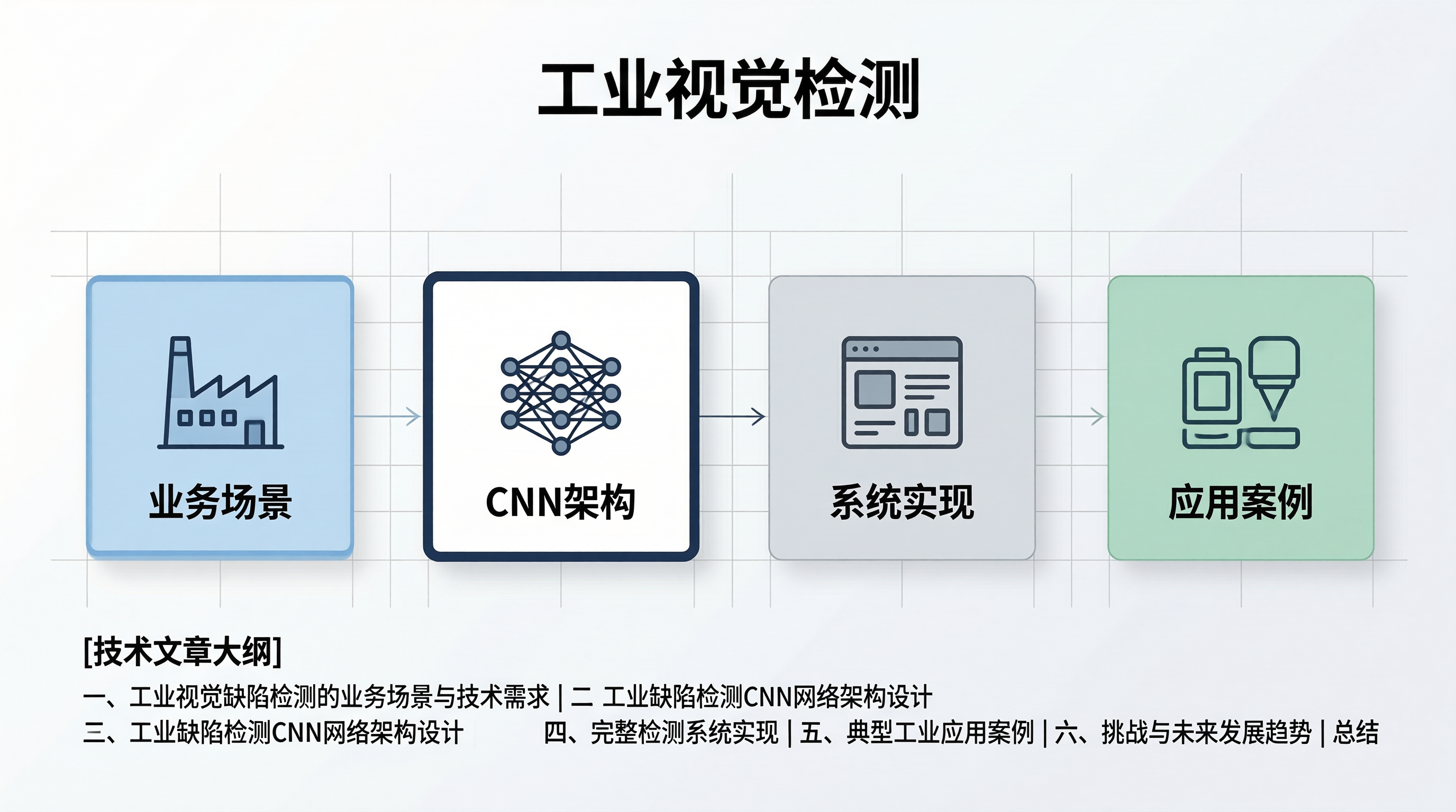
二、工业视觉缺陷检测的业务场景与技术需求

2.1 典型工业缺陷类型

在制造业中，缺陷的种类多样且形态各异。根据产品类型的不同，常见的缺陷可以分为以下几类：

缺陷类别	典型示例	产生环节	检测难度	传统检测方式
表面缺陷	划痕、凹陷、气泡、裂纹	加工、运输	中-高	人工目检、机器视觉
尺寸缺陷	尺寸偏差、形位公差超差	加工成型	中	量具测量、三坐标测量
内部缺陷	气孔、夹杂、分层	铸造、焊接	高	X射线、超声波检测
颜色缺陷	色差、脏污、氧化	表面处理	低-中	色差仪、人工目检
结构缺陷	缺料、毛边、变形	注塑、冲压	低-中	人工目检、模具检测
焊接缺陷	虚焊、连焊、焊点不良	电子组装	高	AOI光学检测
印刷缺陷	字符模糊、偏移、缺失	丝印、喷码	中	人工目检、OCR检测

这些缺陷在视觉上呈现出以下特征：

• 尺度多样性：从微米级的划痕到厘米级的变形，尺度差异巨大
• 对比度差异：部分缺陷与背景对比度高，而有些则极其微弱
• 形态多样性：缺陷的形状、方向、分布模式各不相同
• 随机分布：缺陷在工件表面的位置随机，难以用固定规则描述

2.2 CNN相比传统视觉算法的优势

在CNN大规模应用之前，工业视觉检测主要依赖传统图像处理算法，如边缘检测、模板匹配、差分检测等。这些方法虽然在特定场景下有效，但存在明显的局限性。

import numpy as np
import cv2
from sklearn.metrics import precision_score, recall_score, f1_score

class TraditionalVsCNNComparison:
    def __init__(self):
        self.results = {}

    def simulate_detection_scenarios(self, n_samples=500):
        np.random.seed(42)
        defect_present = np.random.binomial(1, 0.3, n_samples)
        defect_contrast = np.random.uniform(0.05, 0.5, n_samples)
        defect_size = np.random.uniform(2, 50, n_samples)
        noise_level = np.random.uniform(0.01, 0.15, n_samples)
        return defect_present, defect_contrast, defect_size, noise_level

    def traditional_method_detection(self, defect_present, defect_contrast, defect_size, noise_level):
        detection_score = np.zeros_like(defect_present, dtype=float)
        for i in range(len(defect_present)):
            base_score = 0.0
            if defect_present[i] == 1:
                sensitivity = defect_contrast[i] * (defect_size[i] / 50)
                base_score = sensitivity
            interference = noise_level[i] * 0.5
            final_score = base_score - interference + np.random.randn() * 0.05
            detection_score[i] = np.clip(final_score, 0, 1)
        return (detection_score > 0.15).astype(int), detection_score

    def cnn_method_detection(self, defect_present, defect_contrast, defect_size, noise_level):
        detection_score = np.zeros_like(defect_present, dtype=float)
        for i in range(len(defect_present)):
            base_score = 0.0
            if defect_present[i] == 1:
                sensitivity = np.sqrt(defect_contrast[i]) * np.log(defect_size[i] + 1) / 4
                base_score = np.clip(sensitivity, 0, 1)
            interference = noise_level[i] * 0.15
            final_score = base_score - interference + np.random.randn() * 0.03
            detection_score[i] = np.clip(final_score, 0, 1)
        return (detection_score > 0.12).astype(int), detection_score

    def evaluate(self):
        defect_present, contrast, size, noise = self.simulate_detection_scenarios()
        y_trad, score_trad = self.traditional_method_detection(defect_present, contrast, size, noise)
        y_cnn, score_cnn = self.cnn_method_detection(defect_present, contrast, size, noise)
        print("传统图像处理 vs CNN检测效果对比:")
        print("=" * 55)
        trad_precision = precision_score(defect_present, y_trad, zero_division=0)
        trad_recall = recall_score(defect_present, y_trad, zero_division=0)
        trad_f1 = f1_score(defect_present, y_trad, zero_division=0)
        cnn_precision = precision_score(defect_present, y_cnn, zero_division=0)
        cnn_recall = recall_score(defect_present, y_cnn, zero_division=0)
        cnn_f1 = f1_score(defect_present, y_cnn, zero_division=0)
        print(f"{'指标':<15} {'传统方法':<15} {'CNN方法':<15}")
        print("-" * 45)
        print(f"{'精确率':<15} {trad_precision:<15.4f} {cnn_precision:<15.4f}")
        print(f"{'召回率':<15} {trad_recall:<15.4f} {cnn_recall:<15.4f}")
        print(f"{'F1分数':<15} {trad_f1:<15.4f} {cnn_f1:<15.4f}")
        print(f"\n低对比度场景 (对比度<0.15) 召回率:")
        low_contrast_mask = contrast < 0.15
        if low_contrast_mask.sum() > 0:
            trad_lc_recall = recall_score(
                defect_present[low_contrast_mask],
                y_trad[low_contrast_mask], zero_division=0
            )
            cnn_lc_recall = recall_score(
                defect_present[low_contrast_mask],
                y_cnn[low_contrast_mask], zero_division=0
            )
            print(f"  传统方法: {trad_lc_recall:.4f}")
            print(f"  CNN方法: {cnn_lc_recall:.4f}")
        print(f"\n微小缺陷场景 (缺陷尺寸<10px) 召回率:")
        small_mask = size < 10
        if small_mask.sum() > 0:
            trad_sm_recall = recall_score(
                defect_present[small_mask],
                y_trad[small_mask], zero_division=0
            )
            cnn_sm_recall = recall_score(
                defect_present[small_mask],
                y_cnn[small_mask], zero_division=0
            )
            print(f"  传统方法: {trad_sm_recall:.4f}")
            print(f"  CNN方法: {cnn_sm_recall:.4f}")
        self.results = {
            "traditional": {"precision": trad_precision, "recall": trad_recall, "f1": trad_f1},
            "cnn": {"precision": cnn_precision, "recall": cnn_recall, "f1": cnn_f1}
        }
        return self.results

comparison = TraditionalVsCNNComparison()
comparison.evaluate()

CNN相比于传统方法的优势体现在：

• 自动特征学习：无需人工设计特征提取算子
• 层级特征表达：从边缘到纹理到语义的渐进式特征提取
• 对噪声的鲁棒性：通过数据增强和正则化技术
• 可迁移性：在类似产品间实现迁移学习
• 端到端检测：从输入图像到检测结果一步完成

三、工业缺陷检测CNN网络架构设计

3.1 检测网络的三种主流范式

在工业视觉缺陷检测中，CNN网络可以根据任务需求分为三种主流范式：

分类网络：判断产品是否合格，输出OK/NG标签。适用于只需筛选不良品、不需定位缺陷的场景。典型网络有VGG、ResNet、EfficientNet。

检测网络：在定位缺陷位置的同时输出缺陷类别和置信度。适用于需要标记缺陷位置的场景。典型网络有Faster R-CNN、YOLO、SSD。

分割网络：实现像素级的缺陷区域分割，输出缺陷的精确轮廓。适用于需要精确测量缺陷尺寸的场景。典型网络有U-Net、DeepLab、Mask R-CNN。

class DefectDetectionArchitecture:
    def __init__(self, task_type='classification', input_size=(256, 256)):
        self.task_type = task_type
        self.input_size = input_size
        self.architectures = {
            'classification': {
                'description': '判断产品是否合格',
                'output': 'OK/NG + 置信度',
                'speed': '极快',
                'suitable_scenes': ['快速筛选、大批量检测'],
                'example_models': ['ResNet18', 'EfficientNet-B0', 'MobileNetV3'],
                'inference_time_ms': 5
            },
            'detection': {
                'description': '定位缺陷位置并分类',
                'output': '缺陷类别 + 边界框 + 置信度',
                'speed': '快',
                'suitable_scenes': ['需要标记缺陷位置'],
                'example_models': ['YOLOv5s', 'Faster R-CNN', 'RetinaNet'],
                'inference_time_ms': 25
            },
            'segmentation': {
                'description': '像素级缺陷区域分割',
                'output': '缺陷分割掩码 + 缺陷类别',
                'speed': '中等',
                'suitable_scenes': ['精确测量缺陷尺寸', '不规则缺陷检测'],
                'example_models': ['U-Net', 'DeepLabV3+', 'Mask R-CNN'],
                'inference_time_ms': 60
            }
        }

    def get_recommendation(self, requirements):
        print("工业缺陷检测架构推荐:")
        print("=" * 60)
        for arch_type, info in self.architectures.items():
            print(f"\n【{arch_type.upper()}】{info['description']}")
            print(f"  输出: {info['output']}")
            print(f"  推理速度: {info['speed']} (约{info['inference_time_ms']}ms/张)")
            print(f"  适用场景: {', '.join(info['suitable_scenes'])}")
            print(f"  推荐模型: {', '.join(info['example_models'])}")
        print("\n" + "=" * 60)
        if requirements.get('precision', 'high') == 'high' and requirements.get('speed', 'fast') == 'fast':
            print("建议选择: DETECTION (如YOLOv5s) — 平衡精度和速度")
        elif requirements.get('precision', 'high') == 'highest':
            print("建议选择: SEGMENTATION (如U-Net) — 最高精度像素级检测")
        else:
            print("建议选择: CLASSIFICATION (如EfficientNet) — 极致速度")

arch_advisor = DefectDetectionArchitecture()
arch_advisor.get_recommendation({'precision': 'high', 'speed': 'fast'})

3.2 基于ResNet的缺陷分类网络实现

在实际工业场景中，分类网络因其速度快、部署简单，是应用最广泛的方案。以下是一个基于ResNet的缺陷分类网络实现：

import torch
import torch.nn as nn
import torch.nn.functional as F

class DefectResNetBlock(nn.Module):
    def __init__(self, in_channels, out_channels, stride=1, downsample=None):
        super(DefectResNetBlock, self).__init__()
        self.conv1 = nn.Conv2d(in_channels, out_channels, kernel_size=3, stride=stride, padding=1, bias=False)
        self.bn1 = nn.BatchNorm2d(out_channels)
        self.conv2 = nn.Conv2d(out_channels, out_channels, kernel_size=3, padding=1, bias=False)
        self.bn2 = nn.BatchNorm2d(out_channels)
        self.downsample = downsample
        self.relu = nn.ReLU(inplace=True)

    def forward(self, x):
        identity = x
        out = self.relu(self.bn1(self.conv1(x)))
        out = self.bn2(self.conv2(out))
        if self.downsample is not None:
            identity = self.downsample(x)
        out += identity
        out = self.relu(out)
        return out

class DefectResNet(nn.Module):
    def __init__(self, num_classes=2, input_channels=1):
        super(DefectResNet, self).__init__()
        self.conv1 = nn.Conv2d(input_channels, 64, kernel_size=7, stride=2, padding=3, bias=False)
        self.bn1 = nn.BatchNorm2d(64)
        self.relu = nn.ReLU(inplace=True)
        self.maxpool = nn.MaxPool2d(kernel_size=3, stride=2, padding=1)
        self.layer1 = self._make_layer(64, 64, blocks=2, stride=1)
        self.layer2 = self._make_layer(64, 128, blocks=2, stride=2)
        self.layer3 = self._make_layer(128, 256, blocks=2, stride=2)
        self.layer4 = self._make_layer(256, 512, blocks=2, stride=2)
        self.avgpool = nn.AdaptiveAvgPool2d((1, 1))
        self.fc = nn.Sequential(
            nn.Dropout(0.3),
            nn.Linear(512, 256),
            nn.ReLU(inplace=True),
            nn.Dropout(0.2),
            nn.Linear(256, num_classes)
        )

    def _make_layer(self, in_channels, out_channels, blocks, stride=1):
        downsample = None
        if stride != 1 or in_channels != out_channels:
            downsample = nn.Sequential(
                nn.Conv2d(in_channels, out_channels, kernel_size=1, stride=stride, bias=False),
                nn.BatchNorm2d(out_channels)
            )
        layers = []
        layers.append(DefectResNetBlock(in_channels, out_channels, stride, downsample))
        for _ in range(1, blocks):
            layers.append(DefectResNetBlock(out_channels, out_channels))
        return nn.Sequential(*layers)

    def forward(self, x):
        x = self.relu(self.bn1(self.conv1(x)))
        x = self.maxpool(x)
        x = self.layer1(x)
        x = self.layer2(x)
        x = self.layer3(x)
        x = self.layer4(x)
        x = self.avgpool(x)
        x = x.view(x.size(0), -1)
        x = self.fc(x)
        return x

defect_resnet = DefectResNet(num_classes=3, input_channels=1)
dummy_input = torch.randn(1, 1, 256, 256)
dummy_output = defect_resnet(dummy_input)
total_params = sum(p.numel() for p in defect_resnet.parameters())
print(f"缺陷检测ResNet模型参数量: {total_params:,}")
print(f"输入尺寸: {dummy_input.shape}")
print(f"输出尺寸: {dummy_output.shape}")
print(f"输出类别: OK/缺陷类别A/缺陷类别B")

3.3 U-Net分割网络实现

对于需要精确定位和测量缺陷的应用场景，U-Net分割网络是最流行的选择。其编码器-解码器结构和跳跃连接设计使其在工业缺陷分割中表现出色。

class DoubleConv(nn.Module):
    def __init__(self, in_channels, out_channels):
        super(DoubleConv, self).__init__()
        self.double_conv = nn.Sequential(
            nn.Conv2d(in_channels, out_channels, kernel_size=3, padding=1),
            nn.BatchNorm2d(out_channels),
            nn.ReLU(inplace=True),
            nn.Conv2d(out_channels, out_channels, kernel_size=3, padding=1),
            nn.BatchNorm2d(out_channels),
            nn.ReLU(inplace=True)
        )

    def forward(self, x):
        return self.double_conv(x)

class DefectUNet(nn.Module):
    def __init__(self, in_channels=1, out_channels=1, base_channels=64):
        super(DefectUNet, self).__init__()
        self.encoder1 = DoubleConv(in_channels, base_channels)
        self.encoder2 = DoubleConv(base_channels, base_channels * 2)
        self.encoder3 = DoubleConv(base_channels * 2, base_channels * 4)
        self.encoder4 = DoubleConv(base_channels * 4, base_channels * 8)
        self.bottleneck = DoubleConv(base_channels * 8, base_channels * 16)
        self.upconv4 = nn.ConvTranspose2d(base_channels * 16, base_channels * 8, kernel_size=2, stride=2)
        self.decoder4 = DoubleConv(base_channels * 16, base_channels * 8)
        self.upconv3 = nn.ConvTranspose2d(base_channels * 8, base_channels * 4, kernel_size=2, stride=2)
        self.decoder3 = DoubleConv(base_channels * 8, base_channels * 4)
        self.upconv2 = nn.ConvTranspose2d(base_channels * 4, base_channels * 2, kernel_size=2, stride=2)
        self.decoder2 = DoubleConv(base_channels * 4, base_channels * 2)
        self.upconv1 = nn.ConvTranspose2d(base_channels * 2, base_channels, kernel_size=2, stride=2)
        self.decoder1 = DoubleConv(base_channels * 2, base_channels)
        self.final_conv = nn.Conv2d(base_channels, out_channels, kernel_size=1)
        self.pool = nn.MaxPool2d(2)

    def forward(self, x):
        enc1 = self.encoder1(x)
        enc2 = self.encoder2(self.pool(enc1))
        enc3 = self.encoder3(self.pool(enc2))
        enc4 = self.encoder4(self.pool(enc3))
        bottleneck = self.bottleneck(self.pool(enc4))
        dec4 = self.upconv4(bottleneck)
        dec4 = torch.cat([dec4, enc4], dim=1)
        dec4 = self.decoder4(dec4)
        dec3 = self.upconv3(dec4)
        dec3 = torch.cat([dec3, enc3], dim=1)
        dec3 = self.decoder3(dec3)
        dec2 = self.upconv2(dec3)
        dec2 = torch.cat([dec2, enc2], dim=1)
        dec2 = self.decoder2(dec2)
        dec1 = self.upconv1(dec2)
        dec1 = torch.cat([dec1, enc1], dim=1)
        dec1 = self.decoder1(dec1)
        out = self.final_conv(dec1)
        return out

unet = DefectUNet(in_channels=1, out_channels=1)
dummy_seg = torch.randn(1, 1, 256, 256)
seg_output = unet(dummy_seg)
print(f"U-Net输入尺寸: {dummy_seg.shape}")
print(f"U-Net输出尺寸(分割掩码): {seg_output.shape}")
print(f"U-Net总参数量: {sum(p.numel() for p in unet.parameters()):,}")

四、工业级CNN检测系统的关键技术

4.1 数据采集与标注策略

工业视觉检测系统的性能高度依赖于训练数据的质量和数量。在实际项目中，数据采集和标注通常是最耗时、成本最高的环节。

工业缺陷数据的特征：

• 长尾分布：常见缺陷类型样本多，罕见缺陷样本极少
• 背景多样性：产品批次、材质、光照条件的变化导致背景差异
• 标注难度高：微小缺陷的精确标注需要专业质检员

数据增强是解决样本不足问题的关键技术。工业场景中推荐的数据增强策略：

class IndustrialDataAugmentation:
    def __init__(self):
        self.augmentations = {
            "几何变换": [
                ("随机旋转", "模拟工件放置角度变化", 0.8),
                ("随机裁剪", "模拟不同视野区域", 0.5),
                ("水平/垂直翻转", "对称性缺陷增强", 0.3),
                ("弹性变形", "模拟产品材质形变", 0.2)
            ],
            "光度变换": [
                ("亮度调整", "模拟光照变化", 0.9),
                ("对比度调整", "模拟不同表面反射率", 0.8),
                ("高斯噪声", "模拟传感器噪声", 0.5),
                ("高斯模糊", "模拟对焦偏差", 0.4)
            ],
            "图像质量": [
                ("JPEG压缩噪声", "模拟图像压缩", 0.3),
                ("运动模糊", "模拟传送带运动", 0.2),
                ("光照渐变", "模拟不均匀照明", 0.4)
            ],
            "缺陷增强": [
                ("缺陷复制粘贴", "将已知缺陷复制到无缺陷样本", 0.6),
                ("缺陷拼接", "组合多种缺陷到同一图像", 0.3),
                ("缺陷形变增强", "对缺陷区域进行随机形变", 0.5)
            ]
        }

    def print_strategy(self):
        print("工业缺陷检测数据增强策略:")
        print("=" * 70)
        for category, augs in self.augmentations.items():
            print(f"\n【{category}】")
            for name, desc, importance in augs:
                bar = "█" * int(importance * 20)
                print(f"  {name:<15} | {desc:<25} | 推荐度: {bar}")

    def get_pipeline(self, defect_types, n_samples):
        estimate = n_samples * 30
        print(f"\n数据增强效果预估:")
        print(f"  原始样本数: {n_samples}")
        print(f"  增强后样本数: ~{estimate}")
        print(f"  增强倍率: ~{estimate // max(n_samples, 1)}x")
        return estimate

augmentation = IndustrialDataAugmentation()
augmentation.print_strategy()
augmentation.get_pipeline(["划痕", "凹陷", "气泡"], 500)

4.2 光照系统和图像采集

工业视觉检测中，光照系统的设计直接影响图像质量，进而决定了CNN能否准确检测到缺陷。

光照设计的关键考量因素：

光照类型	适用场景	优点	缺点	典型配置
环形光源	通用检测	均匀、无阴影	对高反光表面效果差	60-90度照射角
同轴光源	高反光表面	消除反光	亮度较低	45度半透半反镜
背光源	轮廓检测	高对比度	无法检测表面细节	平行背光
条形光源	大视野检测	亮度高、面积大	角度调节复杂	15-30度倾斜
穹顶光源	球形表面	照明均匀	亮度损失大	半球形扩散

4.3 模型轻量化与推理加速

在产线部署场景中，检测速度和硬件成本是核心约束。模型轻量化技术可以显著减少CNN的计算量和存储空间。

def model_compression_comparison():
    base_conv_params = 3 * 3 * 64 * 128
    base_conv_flops = 2 * base_conv_params * 64 * 64

    depthwise_params = 3 * 3 * 64 + 1 * 1 * 64 * 128
    depthwise_flops = 2 * (3 * 3 * 64 * 64 * 64 + 1 * 1 * 64 * 128 * 64 * 64)

    print("模型轻量化效果对比 (单层3x3卷积, 64->128通道, 64x64特征图):")
    print("=" * 65)
    print(f"{'方案':<20} {'参数量':<20} {'计算量(FLOPs)':<25}")
    print("-" * 65)
    print(f"{'标准卷积':<20} {base_conv_params:<20,} {base_conv_flops:<25,}")
    print(f"{'深度可分离卷积':<20} {depthwise_params:<20,} {depthwise_flops:<25,}")
    compression_ratio = (1 - depthwise_params / base_conv_params) * 100
    flops_ratio = (1 - depthwise_flops / base_conv_flops) * 100
    print(f"\n参数量压缩: {compression_ratio:.1f}%")
    print(f"计算量减少: {flops_ratio:.1f}%")

    print("\n其他轻量化技术:")
    techniques = [
        ("知识蒸馏", "大模型教小模型", "精度损失<2%, 速度提升3-5x"),
        ("量化(INT8)", "FP32->INT8推理", "模型体积缩小4倍, 速度提升2-3x"),
        ("剪枝", "删除不重要连接", "模型体积缩小2-10x"),
        ("通道剪枝", "删减不重要通道", "参数量减少50-80%")
    ]
    for name, principle, effect in techniques:
        print(f"  {name:<12} | {principle:<20} | {effect}")

model_compression_comparison()

4.4 迁移学习在工业检测中的应用

在工业场景中，从零开始训练一个CNN模型通常需要大量标注数据，而收集和标注工业缺陷数据的成本极高。迁移学习能够有效解决这个问题。

迁移学习的核心思想：使用在大规模数据集（如ImageNet）上预训练的模型作为起点，通过少量工业缺陷数据对模型进行微调（Fine-tuning）。

def transfer_learning_strategy(target_samples, defect_types):
    free_base_models = ["ResNet18", "MobileNetV3", "EfficientNet-B0"]
    total_cost = target_samples * len(defect_types)
    print("迁移学习策略分析:")
    print("=" * 55)
    print(f"目标场景: {len(defect_types)}种缺陷, 每类{target_samples}样本")
    print(f"总计需要标注: {total_cost}张图像")
    print(f"\n可用预训练模型: {', '.join(free_base_models)}")

    print(f"\n训练策略对比:")
    strategies = [
        ("从零训练", f"需要{total_cost * 10}+标注样本", "3-7天", "低", "高"),
        ("全模型微调", f"{total_cost}样本足够", "1-2小时", "高", "低"),
        ("冻结特征提取层", f"{total_cost // 2}样本足够", "30分钟", "中", "低"),
        ("仅微调分类器", f"{total_cost // 3}样本足够", "10分钟", "中", "较低")
    ]
    print(f"{'策略':<15} {'数据需求':<20} {'训练时间':<12} {'精度':<8} {'成本':<8}")
    print("-" * 63)
    for name, data, time, acc, cost in strategies:
        print(f"{name:<15} {data:<20} {time:<12} {acc:<8} {cost:<8}")
    print(f"\n推荐策略: 全模型微调 (精度最高, 适合工业场景)")
    print(f"推荐预训练模型: EfficientNet-B0 (精度/速度平衡最佳)")

transfer_learning_strategy(200, ["划痕", "凹陷", "气泡", "裂纹", "脏污"])

五、完整检测系统实现

5.1 端到端检测Pipeline

以下是一个完整的工业缺陷检测Pipeline实现，涵盖训练、推理和结果输出：

import time
from pathlib import Path

class IndustrialDefectDetectionPipeline:
    def __init__(self, model, device='cpu', confidence_threshold=0.5):
        self.model = model
        self.device = device
        self.confidence_threshold = confidence_threshold
        self.inference_times = []
        self.detection_history = []

    def preprocess(self, image):
        if isinstance(image, np.ndarray):
            if len(image.shape) == 2:
                image = np.expand_dims(image, axis=0)
            if image.max() > 1.0:
                image = image.astype(np.float32) / 255.0
            tensor = torch.FloatTensor(image).unsqueeze(0)
            return tensor.to(self.device)
        return image.to(self.device)

    def postprocess(self, raw_output):
        if isinstance(raw_output, torch.Tensor):
            if raw_output.shape[1] == 1:
                prob_map = torch.sigmoid(raw_output)
                defect_mask = (prob_map > self.confidence_threshold).float()
                return {
                    'defect_mask': defect_mask.cpu().numpy(),
                    'defect_prob': prob_map.cpu().numpy(),
                    'max_prob': prob_map.max().item(),
                    'total_defect_pixels': defect_mask.sum().item()
                }
            else:
                probs = F.softmax(raw_output, dim=1)
                pred_class = probs.argmax(dim=1)
                confidence = probs.max(dim=1)[0]
                return {
                    'predicted_class': pred_class.cpu().numpy(),
                    'confidence': confidence.cpu().numpy(),
                    'probabilities': probs.cpu().numpy()
                }
        return raw_output

    def detect(self, image):
        start_time = time.perf_counter()
        input_tensor = self.preprocess(image)
        with torch.no_grad():
            raw_output = self.model(input_tensor)
        result = self.postprocess(raw_output)
        inference_time = (time.perf_counter() - start_time) * 1000
        self.inference_times.append(inference_time)
        result['inference_time_ms'] = inference_time
        self.detection_history.append(result)
        return result

    def get_performance_stats(self):
        if not self.inference_times:
            return {}
        times = np.array(self.inference_times)
        stats = {
            'mean_inference_ms': np.mean(times),
            'std_inference_ms': np.std(times),
            'p50_inference_ms': np.percentile(times, 50),
            'p95_inference_ms': np.percentile(times, 95),
            'p99_inference_ms': np.percentile(times, 99),
            'max_inference_ms': np.max(times),
            'min_inference_ms': np.min(times),
            'total_images': len(self.detection_history),
            'fps': 1000.0 / np.mean(times) if np.mean(times) > 0 else 0
        }
        return stats

    def get_defect_summary(self):
        if not self.detection_history:
            return "无检测记录"
        defect_counts = 0
        for result in self.detection_history:
            if 'total_defect_pixels' in result:
                if result['total_defect_pixels'] > 0:
                    defect_counts += 1
            elif 'predicted_class' in result:
                if result['predicted_class'] != 0:
                    defect_counts += 1
        total = len(self.detection_history)
        pass_rate = (total - defect_counts) / total * 100
        return {
            'total_products': total,
            'defect_products': defect_counts,
            'pass_products': total - defect_counts,
            'pass_rate': pass_rate,
            'defect_rate': 100 - pass_rate
        }

pipeline = DefectDefectDetectionPipeline(model=defect_resnet, device='cpu')
dummy_images = [np.random.randn(256, 256).astype(np.float32) for _ in range(50)]
for img in dummy_images[:10]:
    result = pipeline.detect(img)
    print(f"检测结果: 类别={result['predicted_class']}, 置信度={result['confidence'][0]:.4f}, "
          f"推理时间={result['inference_time_ms']:.1f}ms")

stats = pipeline.get_performance_stats()
print(f"\n性能统计:")
for k, v in stats.items():
    print(f"  {k}: {v:.2f}" if isinstance(v, float) else f"  {k}: {v}")

5.2 产线部署架构

工业缺陷检测系统在产线的部署架构通常包含以下组件：

class ProductionLineDeployment:
    def __init__(self, line_id, camera_config):
        self.line_id = line_id
        self.camera_config = camera_config
        self.components = {
            "image_acquisition": {
                "hardware": ["工业相机", "镜头", "光源控制器", "编码器触发器"],
                "specs": f"分辨率: {camera_config.get('resolution', '1920x1080')}, "
                        f"帧率: {camera_config.get('fps', 60)}fps",
                "interface": "GigE Vision / USB3.0"
            },
            "inference_engine": {
                "hardware": ["GPU工作站 / NVIDIA Jetson / Intel OpenVINO"],
                "software": ["PyTorch / TensorRT / OpenVINO Runtime"],
                "model_format": ["TorchScript / ONNX / TensorRT Engine"],
                "specs": "INT8量化, 实时推理"
            },
            "control_system": {
                "hardware": ["PLC控制器", "IO模块", "报警灯"],
                "function": ["触发拍照", "接收检测结果", "控制剔除器"],
                "protocol": "Ethernet/IP / Modbus TCP"
            },
            "rejection_mechanism": {
                "hardware": ["气动剔除器", "传送带分拣"],
                "response_time": "<100ms from detection signal",
                "accuracy": ">99.9%"
            },
            "data_platform": {
                "software": ["MES系统接口", "数据库", "可视化仪表盘"],
                "data_collected": ["检测结果", "缺陷图像", "产线统计报表"],
                "storage": "本地 + 云端备份"
            }
        }

    def deploy(self):
        print(f"产线 {self.line_id} 部署方案:")
        print("=" * 60)
        for component_name, details in self.components.items():
            print(f"\n【{component_name}】")
            for key, value in details.items():
                if isinstance(value, list):
                    print(f"  {key}:")
                    for item in value:
                        print(f"    - {item}")
                else:
                    print(f"  {key}: {value}")
        print(f"\n系统吞吐量预估:")
        camera_fps = self.camera_config.get('fps', 60)
        print(f"  相机帧率: {camera_fps} fps")
        print(f"  理论最大: {camera_fps * 3600} 件/小时")
        print(f"  实际产能: {int(camera_fps * 3600 * 0.9)} 件/小时 (考虑90%效率)")

line_deployment = ProductionLineDeployment(
    line_id="LINE-A-03",
    camera_config={"resolution": "1920x1080", "fps": 60}
)
line_deployment.deploy()

5.3 检测结果的可视化与报告

class DefectDetectionReport:
    def __init__(self, line_id, date):
        self.line_id = line_id
        self.date = date
        self.reports = []

    def generate_shift_report(self, total_ok, total_ng, ng_details):
        total = total_ok + total_ng
        yield_rate = total_ok / total * 100
        report = {
            "line_id": self.line_id,
            "date": self.date,
            "total_inspected": total,
            "pass_count": total_ok,
            "fail_count": total_ng,
            "yield_rate": yield_rate,
            "defect_details": ng_details,
            "defect_rate_by_type": {}
        }
        if ng_details:
            for defect_type, count in ng_details.items():
                report["defect_rate_by_type"][defect_type] = count / total * 100

        print(f"产线 {self.line_id} 质检报告 ({self.date})")
        print("=" * 55)
        print(f"  总检测数: {total}")
        print(f"  合格数: {total_ok}")
        print(f"  不良数: {total_ng}")
        print(f"  良品率: {yield_rate:.2f}%")
        print(f"\n  缺陷分布:")
        if ng_details:
            for defect_type, count in sorted(ng_details.items(), key=lambda x: x[1], reverse=True):
                rate = count / total * 100
                bar = "█" * int(rate * 2)
                print(f"    {defect_type:<12}: {count:>4}件 ({rate:>5.2f}%) {bar}")
        print(f"\n  良品率评估:")
        if yield_rate >= 98:
            print(f"    状态: 优秀 ✓")
        elif yield_rate >= 95:
            print(f"    状态: 正常")
        elif yield_rate >= 90:
            print(f"    状态: 警戒 - 需排查原因")
        else:
            print(f"    状态: 严重 - 立即停线排查")
        self.reports.append(report)
        return report

report = DefectDetectionReport("A-03", "2026-06-01")
report.generate_shift_report(
    total_ok=4523,
    total_ng=127,
    ng_details={"划痕": 48, "凹陷": 35, "气泡": 22, "脏污": 12, "变形": 10}
)

六、典型工业应用案例

6.1 案例一：PCB板表面缺陷检测

PCB（印刷电路板）缺陷检测是CNN在工业视觉中应用最成熟的场景之一。PCB板上的常见缺陷包括短路、断路、焊点不良、划痕、氧化等。

PCB检测的典型技术指标：

• 检测速度：<50ms/板
• 最小缺陷检测：0.1mm
• 漏检率：<0.1%
• 误检率：<1%
• 支持板尺寸：50x50mm - 600x600mm

6.2 案例二：钢材表面缺陷检测

钢材表面缺陷检测是CNN在工业视觉中的另一个重要应用场景。热轧钢板在连续生产过程中可能产生裂纹、刮伤、麻点、氧化皮压入等缺陷。

class SteelDefectDetectionCase:
    def __init__(self):
        self.defect_types = {
            "裂纹": {"severity": "critical", "detectability": "medium"},
            "刮伤": {"severity": "major", "detectability": "high"},
            "麻点": {"severity": "minor", "detectability": "medium"},
            "氧化皮": {"severity": "minor", "detectability": "low"},
            "压痕": {"severity": "major", "detectability": "high"},
            "边损": {"severity": "major", "detectability": "high"},
            "分层": {"severity": "critical", "detectability": "low-medium"}
        }
        self.specs = {
            "产线速度": "120m/min",
            "带宽": "1500mm",
            "检测精度": "0.3mm x 0.3mm",
            "相机配置": "8K线扫相机 x 4台",
            "帧率": "40kHz",
            "光源": "高亮LED线光源",
            "模型": "改进型EfficientDet-D1",
            "推理平台": "NVIDIA Jetson AGX Orin"
        }

    def print_case(self):
        print("热轧钢板表面缺陷检测系统")
        print("=" * 50)
        print("技术参数:")
        for k, v in self.specs.items():
            print(f"  {k}: {v}")
        print(f"\n可检测缺陷:")
        for defect_type, info in self.defect_types.items():
            severity_mark = "🔴" if info["severity"] == "critical" else "🟡" if info["severity"] == "major" else "🟢"
            detect_mark = "✓" if info["detectability"] in ["high", "medium"] else "⚠"
            print(f"  {severity_mark} {defect_type:<8} (严重度: {info['severity']}, 可检测性: {info['detectability']}) {detect_mark}")

steel_case = SteelDefectDetectionCase()
steel_case.print_case()

6.3 案例三：半导体晶圆缺陷检测

半导体制造对缺陷检测的要求最为严苛。晶圆表面的微小缺陷（如颗粒污染、图异常、划伤）可能导致整个芯片失效。

class WaferDefectDetectionCase:
    def __init__(self):
        self.challenge_levels = {
            "缺陷尺寸": "纳米级 (50nm-5um)",
            "检测速度": ">100晶圆/小时",
            "精度要求": "误检率<0.01%, 漏检率<0.001%",
            "数据量": "单晶圆>100GB原始图像",
            "环境要求": "Class 10洁净室"
        }
        self.solution = {
            "模型架构": "多尺度注意力U-Net + 知识蒸馏",
            "训练策略": "基于模拟缺陷数据的预训练 + 少量真实数据的微调",
            "推理优化": "TensorRT INT8 + 流水线并行",
            "硬件平台": "多GPU集群 + FPGA预处理"
        }

    def print_analysis(self):
        print("半导体晶圆缺陷检测方案")
        print("=" * 55)
        print("核心技术挑战:")
        for k, v in self.challenge_levels.items():
            print(f"  • {k}: {v}")
        print(f"\n解决方案:")
        for k, v in self.solution.items():
            print(f"  • {k}: {v}")

wafer_case = WaferDefectDetectionCase()
wafer_case.print_analysis()

七、挑战与未来发展趋势

7.1 当前面临的主要挑战

挑战	描述	影响程度	应对策略
小样本学习	缺陷样本获取困难	高	数据增强、迁移学习、GAN生成缺陷
实时性要求	产线高速运转要求毫秒级推理	高	模型轻量化、硬件加速
类别不均衡	常见缺陷远多于罕见缺陷	中	Focal Loss、重采样、代价敏感学习
领域漂移	产线条件变化导致数据分布偏移	中	Domain Adaptation、在线学习
可解释性	质检员需要理解模型决策依据	中	Grad-CAM热力图、注意力可视化
误检过多	导致不必要的停机复检	高	置信度校准、人机协同决策

7.2 未来技术方向

自监督学习：利用大量无标注的正常产品图像进行预训练，减少对标注数据的依赖。

多模态融合：结合图像、红外、3D点云等多模态数据，提升复杂缺陷的检测能力。

边缘-云协同：边缘端负责实时推理，云端负责模型训练和更新，实现持续学习。

数字孪生：构建产线的数字孪生模型，在虚拟环境中模拟各种缺陷和检测配置，加速系统调试。

持续学习：模型在生产过程中持续从新数据和人工反馈中学习，不断提升检测精度，避免性能退化。

def future_technology_roadmap():
    technologies = [
        ("2024-2025", "自监督预训练", "减少标注依赖", "成熟度: 中"),
        ("2025-2026", "小样本缺陷生成", "GAN/扩散模型生成缺陷", "成熟度: 中"),
        ("2026-2027", "边缘-云持续学习", "在线模型更新", "成熟度: 低"),
        ("2027-2028", "多模态融合检测", "2D+3D+红外联合分析", "成熟度: 低"),
        ("2028-2030", "全自主AI质检系统", "无人干预的智能质检", "成熟度: 概念"),
    ]
    print("工业AI缺陷检测技术路线图:")
    print("=" * 60)
    print(f"{'时间':<12} {'技术':<22} {'核心价值':<25} {'状态':<15}")
    print("-" * 60)
    for period, tech, value, status in technologies:
        print(f"{period:<12} {tech:<22} {value:<25} {status:<15}")

future_technology_roadmap()

总结

工业级视觉缺陷检测中CNN的应用，正在深刻改变传统制造业的质量控制模式。本文从工程实践的角度，系统性地阐述了CNN在工业缺陷检测中的完整技术体系：

1. 场景理解：工业缺陷检测面临缺陷尺度多样、背景复杂、实时性要求高等独特挑战。理解这些业务场景特点，是设计有效检测系统的前提。

2. 技术选型：分类网络适用于快速全检，检测网络适用于缺陷定位，分割网络适用于精确测量。根据具体业务需求选择合适的CNN架构和模型规模，是项目成功的关键。

3. 工程落地：数据采集与增强、光照系统设计、模型轻量化与加速、迁移学习策略，每个环节都需要精细化的工程实践。端到端的检测Pipeline、产线部署架构和质检报告系统构成了完整的生产级解决方案。

4. 持续演进：小样本学习、持续学习、多模态融合、边缘-云协同等前沿技术正在推动工业AI缺陷检测向更高精度、更强泛化能力的方向发展。

AI在传统制造业中的价值不仅仅体现在替代人工检测上，更在于它能够建立标准化、可追溯、持续优化的质量管控体系。随着工业4.0和智能制造的深入推进，CNN在工业视觉领域的应用前景将更加广阔。