第001/19页（英文原文）

mHC: Manifold-Constrained Hyper-Connections

Zhenda Xie*†, Yixuan Wei*, Huanqi Cao*,

Chenggang Zhao, Chengqi Deng, Jiashi Li, Damai Dai, Huazuo Gao, Jiang Chang, Kuai Yu, Liang Zhao, Shangyan Zhou, Zhean Xu, Zhengyan Zhang, Wangding Zeng, Shengding Hu, Yuqing Wang, Jingyang Yuan, Lean Wang, Wenfeng Liang

DeepSeek-AI

Abstract

Recently, studies exemplified by Hyper-Connections (HC) have extended the ubiquitous residual connection paradigm established over the past decade by expanding the residual stream width and diversifying connectivity patterns. While yielding substantial performance gains, this diversification fundamentally compromises the identity mapping property intrinsic to the residual connection, which causes severe training instability and restricted scalability, and additionally incurs notable memory access overhead. To address these challenges, we propose Manifold-Constrained Hyper-Connections (mHC), a general framework that projects the residual connection space of HC onto a specific manifold to restore the identity mapping property, while incorporating rigorous infrastructure optimization to ensure efficiency. Empirical experiments demonstrate that mHC is effective for training at scale, offering tangible performance improvements and superior scalability. We anticipate that mHC, as a flexible and practical extension of HC, will contribute to a deeper understanding of topological architecture design and suggest promising directions for the evolution of foundational models.

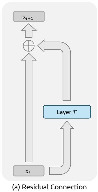
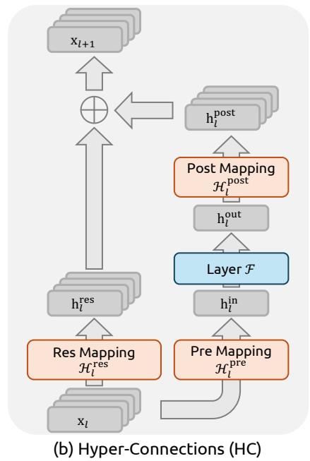
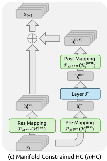
Figure 1 | Illustrations of Residual Connection Paradigms. This figure compares the structural design of (a) standard Residual Connection, (b) Hyper-Connections (HC), and © our proposed Manifold-Constrained Hyper-Connections (mHC). Unlike the unconstrained HC, mHC focuses on optimizing the residual connection space by projecting the matrices onto a constrained manifold to ensure stability.

第001/19页（中文翻译）

$m$ 超连接: 流形约束超连接

Zhenda Xie*†、Yixuan Wei*、Huanqi Cao*、

Chenggang Zhao、Chengqi Deng、Jiashi Li、Damai Dai、Huazuo Gao、Jiang Chang、Kuai Yu、Liang Zhao、Shangyan Zhou、Zhean Xu、Zhengyan Zhang、Wangding Zeng、Shengding Hu、Yuqing Wang、JingyangYuan、Lean Wang、Wenfeng Liang

DeepSeek-AI

摘要

最近，以超连接为代表的研究通过扩展残差流宽度和多样化连接模式，拓展了过去十年建立的普遍存在的残差连接范式。这种多样化虽然带来了显著的性能提升，但根本上损害了残差连接固有的恒等映射性质，从而导致严重的训练不稳定性和受限的可扩展性，并额外产生显著的内存访问开销。为应对这些挑战，我们提出流形约束超连接（mHC），这是一个通用框架，它将超连接的残差连接空间投影到特定流形上以恢复恒等映射性质，同时结合严格的基础设施数优化以确保效率。实证实验表明，mHC对于大规模训练是有效的，能带来切实的性能改进和卓越的可扩展性。我们预期，mHC作为超连接灵活且实用的扩展，将有助于更深入地理解拓扑架构设计，并为基础模型的演进指明有前景的方向。

(a) 残差连接

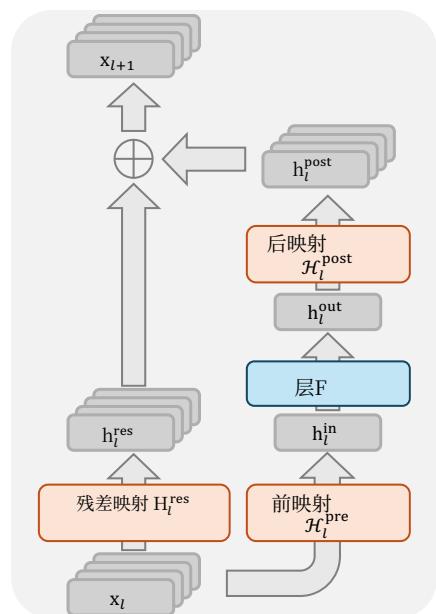
(b) 超连接 (HC)

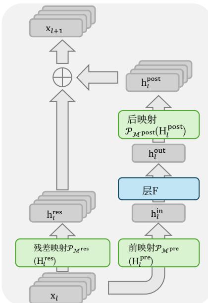
© 流形约束超连接 (mHC)
图1|残差连接范式示意图。本图比较了(a)标准残差连接、(b)超连接以及©我们提出的流形约束超连接(mHC)的结构设计。与无约束的超连接不同，mHC专注于通过将矩阵投影到约束流形上来优化残差连接空间，以确保稳定性。

---

第002/19页（英文原文）

Contents

1 Introduction 3

2 Related Works 4

2.1 Micro Design 4
2.2 Macro Design 5

3 Preliminary 5

3.1 Numerical Instability 6
3.2 System Overhead 7

4 Method 8

4.1 Manifold-Constrained Hyper-Connections 8
4.2 Parameterization and Manifold Projection 9
4.3 Efficient Infrastructure Design 9

4.3.1 Kernel Fusion 9
4.3.2 Recomputing 10
4.3.3 Overlapping Communication in DualPipe 11

5 Experiments 12

5.1 Experimental Setup 12
5.2 Main Results 12
5.3 Scaling Experiments 13
5.4 Stability Analysis 14

6 Conclusion and Outlook 15

A Appendix 19

A.1 Detailed Model Specifications and Hyper-parameters. 19

第002/19页（中文翻译）

目录

1引言32相关工作42.1微观设计.42.2

.53 预备知识 3.1 数值不稳定性.63.2 系统开销.74 方法 84.1 流形约束超连接.84.2 参数化与流形投影.94.3 高效基础设施设计.94.3.1 核融合.94.3.2 重计算.104.3.3 DualPipe中的重叠通信.115 实验 125.1 实验设置.125.2

Main结果

.125.3扩展实验.135.4稳定性分析.146结论与展望15A附录19A.1详细模型规格与超参数.19

---

第003/19页（英文原文）

1. Introduction

Deep neural network architectures have undergone rapid evolution since the introduction of ResNets (He et al., 2016a). As illustrated in Fig. 1(a), the structure of a single-layer can be formulated as follows:

$${\mathbf{x}}_{l+1}={\mathbf{x}}_l+\mathcal{F}({\mathbf{x}}_l,{\mathcal{W}}_l),\text{\hspace{1em}(1)}$$

where ${\mathbf{x}}_l$ and ${\mathbf{x}}_{l+1}$ denote the $C$ -dimensional input and output of the $l$ -th layer, respectively, and $\mathcal{F}$ represents the residual function. Although the residual function $\mathcal{F}$ has evolved over the past decade to include various operations such as convolution, attention mechanisms, and feed forward networks, the paradigm of the residual connection has maintained its original form. Accompanying the progression of Transformer (Vaswani et al., 2017) architecture, this paradigm has currently established itself as a fundamental design element in large language models (LLMs) (Brown et al., 2020; Liu et al., 2024b; Touvron et al., 2023).

This success is primarily attributed to the concise form of the residual connection. More importantly, early research (He et al., 2016b) revealed that the identity mapping property of the residual connection maintains stability and efficiency during large-scale training. By recursively extending the residual connection across multiple layers, Eq. (1) yields:

$${\mathbf{x}}_L={\mathbf{x}}_l+\sum _{i=l}^{L-1}\mathcal{F}\left({\mathbf{x}}_i,{\mathcal{W}}_i\right),\text{\hspace{1em}(2)}$$

where $L$ and $l$ correspond to deeper and shallower layers, respectively. The term identity mapping refers to the component ${\mathbf{x}}_l$ itself, which emphasizes the property that the signal from the shallower layer maps directly to the deeper layer without any modification.

Recently, studies exemplified by Hyper-Connections (HC) (Zhu et al., 2024) have introduced a new dimension to the residual connection and empirically demonstrated its performance potential. The single-layer architecture of HC is illustrated in Fig. 1(b). By expanding the width of the residual stream and enhancing connection complexity, HC significantly increases topological complexity without altering the computational overhead of individual units regarding FLOPs. Formally, single-layer propagation in HC is defined as:

$${\mathbf{x}}_{l+1}={\mathcal{H}}_l^{\mathrm{res}}{\mathbf{x}}_l+{\mathcal{H}}_l^{\mathrm{post}\top }\mathcal{F}({\mathcal{H}}_l^{\mathrm{pre}}{\mathbf{x}}_l,{\mathcal{W}}_l),\text{\hspace{1em}(3)}$$

where ${\mathbf{x}}_l$ and ${\mathbf{x}}_{l+1}$ denote the input and output of the $l$ -th layer, respectively. Unlike the formulation in Eq. (1), the feature dimension of ${\mathbf{x}}_l$ and ${\mathbf{x}}_{l+1}$ is expanded from $C$ to $n\times C$ , where $n$ is the expansion rate. The term ${\mathcal{H}}_l^{\mathrm{res}}\in {\mathbb{R}}^{n\times n}$ represents a learnable mapping that mixes features within the residual stream. Also as a learnable mapping, ${\mathcal{H}}_l^{\mathrm{pre}}\in {\mathbb{R}}^{1\times n}$ aggregates features from the $nC$ -dim stream into a $C$ -dim layer input, and conversely, ${\mathcal{H}}_l^{\mathrm{post}}\in {\mathbb{R}}^{1\times n}$ maps the layer output back onto the stream.

However, as the training scale increases, HC introduces potential risks of instability. The primary concern is that the unconstrained nature of HC compromises the identity mapping property when the architecture extends across multiple layers. In architectures comprising multiple parallel streams, an ideal identity mapping serves as a conservation mechanism. It ensures that the average signal intensity across streams remains invariant during both forward and backward propagation. Recursively extending HC to multiple layers via Eq. (3) yields:

$${\mathbf{x}}_L=\left(\prod _{i=1}^{L-l}{\mathcal{H}}_{L-i}^{\text{r e s}}\right){\mathbf{x}}_l+\sum _{i=l}^{L-1}\left(\prod _{j=1}^{L-1-i}{\mathcal{H}}_{L-j}^{\text{r e s}}\right){\mathcal{H}}_i^{\text{p o s t}\top }\mathcal{F}\left({\mathcal{H}}_i^{\text{p r e}}{\mathbf{x}}_i,{\mathcal{W}}_i\right),\text{\hspace{1em}(4)}$$

第003/19页（中文翻译）

1. 引言

自ResNets（He等，2016a）被提出以来，深度神经网络架构经历了快速的演变。如图1(a)所示，单层的结构可以表述如下：

$${\mathbf{x}}_{l+1}={\mathbf{x}}_l+\mathcal{F}\left({\mathbf{x}}_l,{\mathcal{W}}_l\right),\text{\hspace{1em}(1)}$$

其中 ${\mathbf{x}}_l$ 和 ${\mathbf{x}}_{l+1}$ 分别表示第 $l$ 层的 $C$ 维输入和输出，F代表残差函数。尽管在过去十年中，残差函数F已演变为包含卷积、注意力机制和前馈网络等多种操作，但残差连接的范式始终保持其原始形式。随着Transformer（Vaswani等，2017）架构的发展，这种范式目前已成为大语言模型（LLMs）（Brown等，2020；Liu等，2024b；Touvron等，2023）中的一项基本设计要素。

这一成功主要归功于残差连接简洁的形式。更重要的是，早期研究（He等，2016b）揭示，残差连接的恒等映射性质在大规模训练期间保持了稳定性和效率。通过将残差连接递归地扩展到多层，公式(1)可推导出：

$${\mathbf{x}}_L={\mathbf{x}}_l+\sum _{i=l}^{L-1}\mathcal{F}\left({\mathbf{x}}_i,{\mathcal{W}}_i\right),\text{\hspace{1em}(2)}$$

其中 $L$ 和 $l$ 分别对应更深的层和更浅的层。术语恒等映射指的是分量 ${\mathbf{x}}_l$ 本身，它强调了来自较浅层的信号无需任何修改直接映射到较深层的特性。

最近，以超连接（Zhu等，2024）为代表的研究为残差连接引入了新的维度，并通过实验证明了其性能潜力。HC的单层架构如图1(b)所示。通过扩展残差流的宽度并增强连接复杂性，HC在不改变单个单元关于浮点运算次数的计算开销的情况下，显著增加了拓扑复杂性。形式上，HC中的单层传播定义为：

$${\mathbf{x}}_{l+1}={\mathcal{H}}_l^{\mathrm{res}}{\mathbf{x}}_l+{\mathcal{H}}_l^{\mathrm{post}\top }\mathcal{F}\left({\mathcal{H}}_l^{\mathrm{pre}}{\mathbf{x}}_l,{\mathcal{W}}_l\right),\text{\hspace{1em}(3)}$$

其中 ${\mathbf{x}}_l$ 和 ${\mathbf{x}}_{l+1}$ 分别表示第 $l$ 层的输入和输出。与公式(1)中的形式不同， ${\mathbf{x}}_l$ 和 ${\mathbf{x}}_{l+1}$ 的特征维度从 $C$ 扩展到 $n\times C$ ，其中 $n$ 是扩展率。项 ${\mathcal{H}}_l^{\mathrm{res}}\in {\mathbb{R}}^{n\times n}$ 代表一个在残差流内混合特征的可学习映射。同样作为可学习映射， ${\mathcal{H}}_l^{\mathrm{pre}}\in {\mathbb{R}}^{1\times n}$ 将来自 $nC$ 维流的特征聚合为 $C$ 维的层输入，反之， ${\mathcal{H}}_l^{\mathrm{post}}\in {\mathbb{R}}^{1\times n}$ 将层输出映射回流上。

然而，随着训练规模扩大，超连接引入了潜在的不稳定性风险。其主要问题在于，当架构扩展到多层时，超连接的无约束特性会损害恒等映射性质。在包含多个并行流的架构中，理想的恒等映射充当一种守恒机制。它确保各流间的平均信号强度在前向传播和反向传播期间保持不变。通过公式（3）将超连接递归扩展到多层会得到：

$${\mathbf{x}}_L=\left(\prod _{i=1}^{L-l}{\mathcal{H}}_{L-i}^{\text{r e s}}\right){\mathbf{x}}_l+\sum _{i=l}^{L-1}\left(\prod _{j=1}^{L-1-i}{\mathcal{H}}_{L-j}^{\text{r e s}}\right){\mathcal{H}}_i^{\text{p o s t}\top }\mathcal{F}\left({\mathcal{H}}_i^{\text{p r e}}{\mathbf{x}}_i,{\mathcal{W}}_i\right),\text{\hspace{1em}(4)}$$

---

第004/19页（英文原文）

where $L$ and $l$ represent a deeper layer and a shallower layer, respectively. In contrast to Eq. (2), the composite mapping ${\prod }_{i=1}^{L-l}{\mathcal{H}}_{L-i}^{\mathrm{res}}$ in HC fails to preserve the global mean of the features. This discrepancy leads to unbounded signal amplification or attenuation, resulting in instability during large-scale training. A further consideration is that, while HC preserves computational efficiency in terms of FLOPs, the hardware efficiency concerning memory access costs for the widened residual stream remains unaddressed in the original design. These factors collectively restrict the practical scalability of HC and hinder its application in large-scale training.

To address these challenges, we propose Manifold-Constrained Hyper-Connections (mHC), as shown in Fig. 1©, a general framework that projects the residual connection space of HC onto a specific manifold to restore the identity mapping property, while incorporating rigorous infrastructure optimization to ensure efficiency. Specifically, mHC utilizes the Sinkhorn-Knopp algorithm (Sinkhorn and Knopp, 1967) to entropically project ${\mathcal{H}}_l^{\mathrm{res}}$ onto the Birkhoff polytope. This operation effectively constrains the residual connection matrices within the manifold that is constituted by doubly stochastic matrices. Since the row and column sums of these matrices equal to 1, the operation ${\mathcal{H}}_l^{\mathrm{res}}{\mathbf{x}}_l$ functions as a convex combination of the input features. This characteristic facilitates a well-conditioned signal propagation where the feature mean is conserved, and the signal norm is strictly regularized, effectively mitigating the risk of vanishing or exploding signals. Furthermore, due to the closure of matrix multiplication for doubly stochastic matrices, the composite mapping ${\prod }_{i=1}^{L-l}{\mathcal{H}}_{L-i}^{\mathrm{res}}$ retains this conservation property. Consequently, mHC effectively maintains the stability of identity mappings between arbitrary depths. To ensure efficiency, we employ kernel fusion and develop mixed precision kernels utilizing TileLang (Wang et al., 2025). Furthermore, we mitigate the memory footprint through selective recomputing and carefully overlap communication within the DualPipe schedule (Liu et al., 2024b).

Extensive experiments on language model pretraining demonstrate that mHC exhibits exceptional stability and scalability while maintaining the performance advantages of HC. In-house large-scale training indicates that mHC supports training at scale and introduces only a $6.7\%$ additional time overhead when expansion rate $n=4$ .

2. Related Works

Architectural advancements in deep learning can be primarily classified into micro-design and macro-design. Micro-design concerns the internal architecture of computational blocks, specifying how features are processed across spatial, temporal, and channel dimensions. In contrast, macro-design establishes the inter-block topological structure, thereby dictating how feature representations are propagated, routed, and merged across distinct layers.

2.1. Micro Design

Driven by parameter sharing and translation invariance, convolution initially dominated the processing of structured signals. While subsequent variations such as depthwise separable (Chollet, 2017) and grouped convolutions (Xie et al., 2017) optimized efficiency, the advent of Transformers (Vaswani et al., 2017) established Attention and Feed-Forward Networks (FFNs) as the fundamental building blocks of modern architecture. Attention mechanisms facilitate global information propagation, while FFNs enhance the representational capacity of individual features. To balance performance with the computational demands of LLMs, attention mechanisms have evolved towards efficient variants such as Multi-Query Attention (MQA) (Shazeer, 2019), Grouped-Query Attention (GQA) (Ainslie et al., 2023), and Multi-Head Latent Attention

第004/19页（中文翻译）

其中 $L$ 和 $l$ 分别代表更深的层和更浅的层。与公式（2）相比，超连接中的复合映射 ${\prod }_{i=1}^{L-l}{\mathcal{H}}_{L-i}^{\mathrm{res}}$ 未能保持特征的全局均值。这种差异会导致信号无限制地放大或衰减，从而在大规模训练中引发不稳定性。另一个需要考虑的因素是，尽管超连接在浮点运算次数方面保持了计算效率，但其原始设计并未解决加宽的残差流所带来的内存访问开销相关的硬件效率问题。这些因素共同限制了超连接的实际可扩展性，并阻碍了其在大规模训练中的应用。

为应对这些挑战，我们提出了流形约束超连接（mHC），如图1©所示。这是一个通用框架，它将HC的残差连接空间投影到特定流形上，以恢复恒等映射性质，同时结合严格的基础设施优化以确保效率。具体来说，mHC利用Sinkhorn-Knopp算法（Sinkhorn和Knopp,1967）将 ${\mathrm{H}}_l^{\mathrm{res}}$ 熵投影到Birkhoff多面体上。此手术有效地将残差连接矩阵约束在由双随机矩阵构成的流形内。由于这些矩阵的行和与列和均等于1，该操作 ${\mathcal{H}}_l^{\mathrm{res}}{\mathbf{x}}_l$ 起到了输入特征凸组合的作用。这一特性促进了信号的良好传播，其中特征均值得以保持，信号范数受到严格正则化，从而有效缓解了信号消失或爆炸的风险。此外，由于双随机矩阵对矩阵乘法的封闭性，复合映射 ${\prod }_{i=1}^{L-l}{\mathcal{H}}_{L-i}^{\mathrm{res}}$ 保留了这一守恒性质。因此，mHC有效地维持了任意深度之间恒等映射的稳定性。为确保效率，我们采用核融合并利用TileLang（Wang等人，2025）开发了混合精度内核。此外，我们通过选择性重计算来减少内存占用，并在DualPipe调度（Liu等，2024b）中精心重叠通信。

在语言模型预训练上的大量实验表明，mHC展现出卓越的稳定性和可扩展性，同时保持了HC的性能优势。内部大规模训练表明，mHC支持大规模训练，并且在扩展率 $n=4$ 时仅引入 $6.7\%$ 的额外时间开销。

2. 相关工作

深度学习的架构进步主要可分为微观设计和宏观设计。微观设计关注计算区块的内部架构，规定了特征在空间、时间和通道维度上如何处理。相反，宏观设计确立了区块间的拓扑结构，从而决定了特征表示如何在不同的层之间传播、路由和合并。

2.1. 微观设计

受参数共享和平移不变性驱动，卷积最初主导了结构化信号的处理。尽管后续出现了深度可分离卷积（Chollet, 2017）和分组卷积（Xie等, 2017）等变体以优化效率，但Transformer（Vaswani等, 2017）的出现确立了注意力机制和前馈网络作为现代架构的基本构建块。注意力机制促进了全局信息传播，而FFN则增强了单个特征的表示能力。为了在性能与大语言模型的计算需求之间取得平衡，注意力机制已演变为高效变体，例如多查询注意力（Shazeer, 2019）、分组查询注意力（Ainslie等, 2023）以及多头潜在注意力。

---

第005/19页（英文原文）

(MLA) (Liu et al., 2024a). Simultaneously, FFNs have been generalized into sparse computing paradigms via Mixture-of-Experts (MoE) (Fedus et al., 2022; Lepikhin et al., 2020; Shazeer et al., 2017), allowing for massive parameter scaling without proportional computational costs.

2.2. Macro Design

Macro-design governs the global topology of the network (Srivastava et al., 2015). Following ResNet (He et al., 2016a), architectures such as DenseNet (Huang et al., 2017) and FractalNet (Larsson et al., 2016) aimed to enhance performance by increasing topological complexity through dense connectivity and multi-path structures, respectively. Deep Layer Aggregation (DLA) (Yu et al., 2018) further extended this paradigm by recursively aggregating features across various depths and resolutions.

More recently, the focus of macro-design has shifted toward expanding the width of the residual stream (Chai et al., 2020; Fang et al., 2023; Heddes et al., 2025; Mak and Flanigan, 2025; Menghani et al., 2025; Pagliardini et al., 2024; Xiao et al., 2025; Xie et al., 2023; Zhu et al., 2024). Hyper-Connections (HC) (Zhu et al., 2024) introduced learnable matrices to modulate connection strengths among features at varying depths, while the Residual Matrix Transformer (RMT) (Mak and Flanigan, 2025) replaced the standard residual stream with an outer-product memory matrix to facilitate feature storage. Similarly, MUFFFormer (Xiao et al., 2025) employs multiway dynamic dense connections to optimize cross-layer information flow. Despite their potential, these approaches compromise the inherent identity mapping property of the residual connection, thereby introducing instability and hindering scalability. Furthermore, they incur significant memory access overhead due to expanded feature widths. Building upon HC, the proposed mHC restricts the residual connection space onto a specific manifold to restore the identity mapping property, while also incorporating rigorous infrastructure optimizations to ensure efficiency. This approach enhances stability and scalability while maintaining the topological benefits of expanded connections.

3. Preliminary

We first establish the notation used in this work. In the HC formulation, the input to the $l$ -th layer, ${\mathbf{x}}_l\in {\mathbb{R}}^{1\times C}$ , is expanded by a factor of $n$ to construct a hidden matrix ${\mathbf{x}}_l=({\mathbf{x}}_{l,0^{\prime }}^{\top },\dots ,{\mathbf{x}}_{l,n-1}^{\top }{)}^{\top }\in {\mathbb{R}}^{n\times C}$ which can be viewed as $n$ -stream residual. This operation effectively broadens the width of the residual stream. To govern the read-out, write-in, and updating processes of this stream, HC introduces three learnable linear mappings— ${\mathcal{H}}_l^{\mathrm{pre}}$ , ${\mathcal{H}}_l^{\mathrm{post}}\in {\mathbb{R}}^{1\times n}$ , and ${\mathcal{H}}_l^{\mathrm{res}}\in {\mathbb{R}}^{n\times n}$ . These mappings modify the standard residual connection shown in Eq. (1), resulting in the formulation given in Eq. (3).

In the HC formulation, learnable mappings are composed of two parts of coefficients: the input-dependent one and the global one, referred to as dynamic mappings and static mappings, respectively. Formally, HC computes the coefficients as follows:

$$\{\begin{array}{l}{\tilde{\mathbf{x}}}_l=\mathrm{RMSNorm}\left({\mathbf{x}}_l\right)\\ {\mathcal{H}}_l^{\text{p r e}}={\alpha }_l^{\text{p r e}}\cdot \tanh \left({\theta }_l^{\text{p r e}}{\tilde{\mathbf{x}}}_l^{\top }\right)+{\mathbf{b}}_l^{\text{p r e}}\\ {\mathcal{H}}_l^{\text{p o s t}}={\alpha }_l^{\text{p o s t}}\cdot \tanh \left({\theta }_l^{\text{p o s t}}{\tilde{\mathbf{x}}}_l^{\top }\right)+{\mathbf{b}}_l^{\text{p o s t}}\\ {\mathcal{H}}_l^{\text{r e s}}={\alpha }_l^{\text{r e s}}\cdot \tanh \left({\theta }_l^{\text{r e s}}{\tilde{\mathbf{x}}}_l^{\top }\right)+{\mathbf{b}}_l^{\text{r e s}},\end{array}\text{\hspace{1em}(5)}$$

where $\mathrm{RMSNorm}(\cdot )$ (Zhang and Sennrich, 2019) is applied to the last dimension, and the scalars ${\alpha }_l^{\mathrm{pre}},{\alpha }_l^{\mathrm{post}}$ and ${\alpha }_l^{\mathrm{res}}\in \mathbb{R}$ are learnable gating factors initialized to small values. The dynamic

第005/19页（中文翻译）

同时，前馈网络已通过专家混合（Fedus等，2022; Lepikhin等，2020; Shazeer等，2017）泛化为稀疏计算范式，允许大规模参数扩展而无需成比例的计算成本。

2.2.宏观设计

宏观设计决定了网络的全局拓扑结构 (Srivastava et al., 2015)。继残差网络 (He 等, 2016a) 之后，诸如密集连接网络 (Huang et al., 2017) 和分形网络 (Larsson et al., 2016) 等架构分别试图通过密集连接和多路径结构来增加拓扑复杂性，从而提升性能。深度层聚合 (Yu et al., 2018) 通过递归聚合不同深度和分辨率下的特征，进一步扩展了这一范式。

最近，宏观设计的重点已转向扩展残差流的宽度 (Chai et al., 2020; Fang et al., 2023; Heddes et al., 2025; Mak and Flanigan, 2025; Menghani et al., 2025; Pagliardini et al., 2024; Xiao et al., 2025; Xie et al., 2023; Zhu等, 2024)。超连接 (Zhu等, 2024) 引入了可学习矩阵来调节不同深度特征间的连接强度，而残差矩阵Transformer (Mak and Flanigan, 2025) 则用外积记忆矩阵取代了标准的残差流，以促进特征存储。类似地，MUDDFormer (Xiao et al., 2025) 采用多路动态密集连接来优化跨层信息流。尽管这些方法具有潜力，但它们牺牲了残差连接固有的恒等映射性质，从而引入了不稳定性并阻碍了可扩展性。此外，由于特征宽度的扩展，它们还产生了显著的内存访问开销。基于超连接，所提出的 mHC 将残差连接空间限制在特定的流形上，以恢复恒等映射性质，同时结合了严格的基础设施数优化以确保效率。这种方法在保持扩展连接拓扑优势的同时，增强了稳定性和可扩展性。

3. 预备知识

我们首先建立本工作中使用的符号。在超连接公式中，第 $l$ 层的输入 ${\mathbf{x}}_l\in {\mathbb{R}}^{1\times C}$ 会被扩展 $n$ 倍，以构建一个可被视为 $n$ 流残差的隐层矩阵 ${\mathbf{x}}_l=({\mathbf{x}}_{l,0}^{\prime },\dots ,{\mathbf{x}}_{l,n-1}^{\prime }{)}^{\top }\in {\mathbb{R}}^{n\times C}$ 。此操作有效地拓宽了残差流的宽度。为了控制此流的读取、写入和更新过程，超连接引入了三个可学习线性映射一 ${\mathcal{H}}_l^{\mathrm{pre}}{\mathcal{H}}_l^{\mathrm{post}}\in {\mathbb{R}}^{1\times n}$ 、 ${\mathcal{H}}_l^{\mathrm{res}}\in {\mathbb{R}}^{n\times n}$ 。这些映射修改了公式(1)所示的标准残差连接，从而得到公式(3)中的表述。

在HCformulation中，可学习映射由两部分系数组成：依赖于输入的部分和全局部分，分别称为动态映射和静态映射。形式上，超连接按如下方式计算系数：

$$\{\begin{array}{l}{\tilde{\mathbf{x}}}_l=\mathrm{RMSNorm}\left({\mathbf{x}}_l\right)\\ {\mathcal{H}}_l^{\text{p r e}}={\alpha }_l^{\text{p r e}}\cdot \tanh \left({\theta }_l^{\text{p r e}}{\tilde{\mathbf{x}}}_l^{\top }\right)+{\mathbf{b}}_l^{\text{p r e}}\\ {\mathcal{H}}_l^{\text{p o s t}}={\alpha }_l^{\text{p o s t}}\cdot \tanh \left({\theta }_l^{\text{p o s t}}{\tilde{\mathbf{x}}}_l^{\top }\right)+{\mathbf{b}}_l^{\text{p o s t}}\\ {\mathcal{H}}_l^{\text{r e s}}={\alpha }_l^{\text{r e s}}\cdot \tanh \left({\theta }_l^{\text{r e s}}{\tilde{\mathbf{x}}}_l^{\top }\right)+{\mathbf{b}}_l^{\text{r e s}},\end{array}\text{\hspace{1em}(5)}$$

其中RMSNorm(·) (Zhang and Sennrich, 2019)应用于最后一个维度，标量 ${\alpha }_l^{\mathrm{pre}}{\alpha }_l^{\mathrm{post}}$ 和 ${\alpha }_l^{\mathrm{res}}\in \mathbb{R}$ 是初始化为较小值的可学习门控因子。动态

---

第006/19页（英文原文）

mappings are derived via linear projections parameterized by ${\theta }_l^{\mathrm{pre}},{\theta }_l^{\mathrm{post}}\in {\mathbb{R}}^{1\times C}$ and ${\theta }_l^{\mathrm{res}}\in {\mathbb{R}}^{n\times C}$ , while the static mappings are represented by learnable biases ${\mathbf{b}}_l^{\mathrm{pre}},{\mathbf{b}}_l^{\mathrm{post}}\in {\mathbb{R}}^{1\times n}$ and ${\mathbf{b}}_l^{\mathrm{res}}\in {\mathbb{R}}^{n\times n}$ .

It is worth noting that the introduction of these mappings— ${\mathcal{H}}_l^{\mathrm{pre}}$ , ${\mathcal{H}}_l^{\mathrm{post}}$ , and ${\mathcal{H}}_l^{\mathrm{res}}$ —incurs negligible computational overhead, as the typical expansion rate $n$ , e.g. 4, is much smaller than the input dimension $C$ . With this design, HC effectively decouples the information capacity of the residual stream from the layer’s input dimension, which is strongly correlated with the model’s computational complexity (FLOPs). Consequently, HC offers a new avenue for scaling by adjusting the residual stream width, complementing the traditional scaling dimensions of model FLOPs and training data size discussed in pre-training scaling laws (Hoffmann et al., 2022).

Although HC necessitates three mappings to manage the dimensional mismatch between the residual stream and the layer input, preliminary experiments presented in Tab. 1 indicate that the residual mapping ${\mathcal{H}}_l^{\mathrm{res}}$ yields the most significant performance gain. This finding underscores the critical importance of effective information exchange within the residual stream.

Table 1 | Ablation Study of HC Components. When a specific mapping $({\mathcal{H}}_l^{\mathrm{pre}},{\mathcal{H}}_l^{\mathrm{post}},$ or ${\mathcal{H}}_l^{\mathrm{res}})$ is disabled, we employ a fixed mapping to maintain dimensional consistency: uniform weights of $1/n$ for ${\mathcal{H}}_l^{\mathrm{pre}}$ , uniform weights of ones for ${\mathcal{H}}_l^{\mathrm{post}}$ , and the identity matrix for ${\mathcal{H}}_l^{\mathrm{res}}$ .

Hlres	Hlpre	Hlpost	Absolute Loss Gap
			0.0
✓			-0.022
✓	✓		-0.025
✓	✓	✓	-0.027

3.1. Numerical Instability

While the residual mapping ${\mathcal{H}}_l^{\mathrm{res}}$ is instrumental for performance, its sequential application poses a significant risk to numerical stability. As detailed in Eq. (4), when HC is extended across multiple layers, the effective signal propagation from layer $l$ to $L$ is governed by the composite mapping ${\prod }_{i=1}^{L-l}{\mathcal{H}}_{L-i}^{\mathrm{res}}$ . Since the learnable mapping ${\mathcal{H}}_l^{\mathrm{res}}$ is unconstrained, this composite mapping inevitably deviates from the identity mapping. Consequently, the signal magnitude is prone to explosion or vanishing during both the forward pass and backpropagation. This phenomenon undermines the fundamental premise of residual learning, which relies on unimpeded signal flow, thereby destabilizing the training process in deeper or larger-scale models.

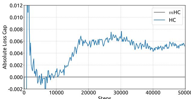
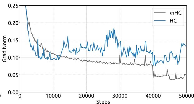
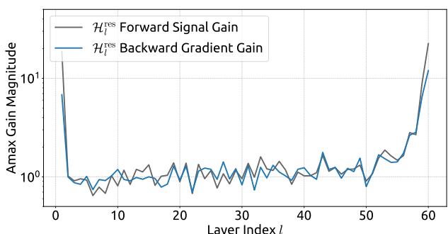
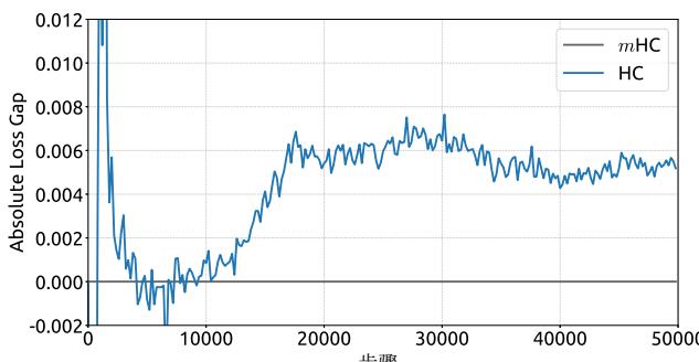
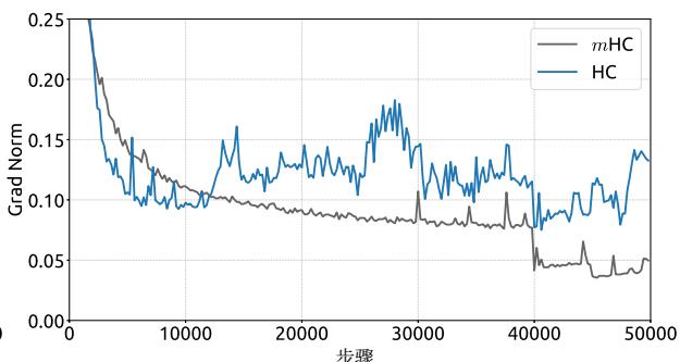
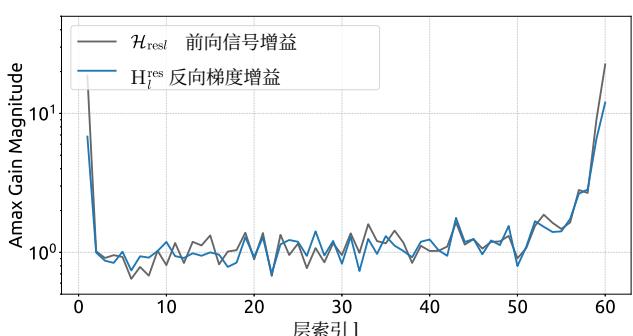
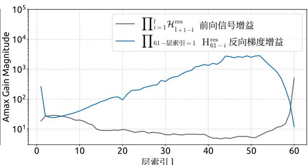
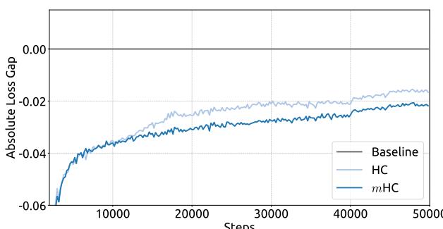
Empirical evidence supports this analysis. We observe unstable loss behavior in large-scale experiments, as illustrated in Fig. 2. Taking mHC as the baseline, HC exhibits an unexpected loss surge around the 12k step, which is highly correlated with the instability in the gradient norm. Furthermore, the analysis on ${\mathcal{H}}_l^{\mathrm{res}}$ validates the mechanism of this instability. To quantify how the composite mapping ${\prod }_{i=1}^{L-l}{\mathcal{H}}_{L-i}^{\mathrm{res}}$ amplifies signals along the residual stream, we utilize two metrics. The first, based on the maximum absolute value of the row sums of the composite mapping, captures the worst-case expansion in the forward pass. The second, based on the maximum absolute column sum, corresponds to the backward pass. We refer to these metrics as the Amax Gain Magnitude of the composite mapping. As shown in Fig. 3(b), the Amax Gain Magnitude yields extreme values with peaks of 3000, a stark divergence from 1 that confirms the presence of exploding residual streams.

第006/19页（中文翻译）

映射通过由 $\theta \mathrm{pre}l$ 、 $\theta {\mathrm{post}}_l\in {\mathbb{R}}^{1\times C}$ 和 $\theta {\mathrm{res}}_l\in {\mathbb{R}}^{n\times C}$ 参数化的线性投影推导得出，而静态映射则由可学习偏置 ${\mathbf{b}}_l^{\mathrm{pre}}{\mathbf{b}}_l^{\mathrm{post}}\in {\mathbb{R}}^{1\times n}$ 和 ${\mathbf{b}}_l^{\mathrm{res}}\in {\mathbb{R}}^{n\times n}$ 表示。

值得注意的是，引入这些映射——H pre $l$ 、H post $l$ 和 ${\mathrm{H}}_l^{\mathrm{res}}$ ——所产生的计算开销可以忽略不计，因为典型的扩展率 $n$ （例如4）远小于输入维度 $C$ 。通过这种设计，HC有效地将残差流的信息容量与层的输入维度解耦，而后者与模型的计算复杂度（浮点运算次数）高度相关。因此，HC通过调整残差流宽度，为模型扩展提供了一条新途径，这补充了预训练扩展律（Hoffmann等人，2022）中讨论的传统扩展维度——模型浮点运算次数和训练数据规模。

尽管HC需要三个映射来处理残差流与层输入之间的维度不匹配，但表1中的初步实验表明，残差映射 ${\mathrm{H}}_l^{\mathrm{res}}$ 带来了最显著的性能提升。这一发现突显了残差流内有效信息交换的至关重要性。

表 1 |HC组件的消融实验。当禁用特定映射 $({\mathrm{H}}_l^{\mathrm{pre}}$ 、 ${\mathrm{H}}_l^{\mathrm{post}}$ 或 $\mathrm{H}\mathrm{res}l)$ 时，我们采用固定的映射来保持维度一致性：为 $\mathrm{H}\mathrm{pre}l$ 使用 $1/n$ 的均匀权重，为 ${\mathcal{H}}_l^{\mathrm{post}}$ 使用全1的均匀权重，并为 ${\mathrm{H}}_l^{\mathrm{res}}$ 使用单位矩阵。

H分辨率l	H前置l	H后置l	绝对损失差距
			0.0
✓			-0.022
✓	✓		-0.025
✓	✓	✓	-0.027

3.1.数值不稳定性

尽管残差映射 ${\mathrm{H}}_l^{\mathrm{res}}$ 对性能至关重要，但其顺序应用对数值稳定性构成了重大风险。如公式（4）所述，当超连接跨越多个层时，从第 $l$ 层到第 $L$ 层的有效信号传播由复合映射 ${\prod }_{i=1}^{L-l}{\mathcal{H}}_{L-i}^{\mathrm{res}}$ 决定。由于可学习映射 $\mathrm{H}$ 是无约束的，此复合映射不可避免地会偏离恒等映射。因此，在前向传播和反向传播过程中，信号幅度容易发生爆炸或消失。这种现象破坏了残差学习的基本前提——即依赖无阻碍的信号流，从而在更深或更大规模的模型中使训练过程变得不稳定。

经验证据支持这一分析。我们在大规模实验中观察到不稳定的损失行为，如图2所示。以 $m$ 超连接为基线，超连接在约12k步长附近出现了意外的损失激增，这与梯度范数的不稳定性高度相关。此外，对 ${\mathcal{H}}_l^{\mathrm{res}}$ 的分析验证了这种不稳定性的机制。为了量化复合映射 ${\prod }_{i=1}^{L-l}{\mathcal{H}}_{L-i}^{\mathrm{res}}$ 如何放大残差流中的信号，我们采用了两个指标。第一个指标基于复合映射行和的最大绝对值，捕捉了前向传播中最坏情况下的扩张。第二个指标基于最大绝对列和，对应于反向传播。我们将这些指标称为复合映射的Amax增益幅度。如图3(b)所示，Amax增益幅度产生了极端值，峰值高达3000，与数值1的显著偏离证实了爆炸性残差流的存在。

---

第007/19页（英文原文）

(a) Absolute Training Loss Gap vs. Training Steps

(b) Gradient Norm vs. Training Steps

(a) Single-Layer Mapping
Figure 3 | Propagation Instability of Hyper-Connections (HC). This figure illustrates the propagation dynamics of (a) the single-layer mapping ${\mathcal{H}}_l^{\mathrm{res}}$ and (b) the composite mapping ${\prod }_{i=1}^{L-l}{\mathcal{H}}_{L-i}^{\mathrm{res}}$ within the 27B model. The layer index $l$ (x-axis) unrolls each standard Transformer block into two independent layers (Attention and FFN). The Amax Gain Magnitude (y-axis) is calculated as the maximum absolute row sum (for the forward signal) and column sum (for the backward gradient), averaged over all tokens in a selected sequence.

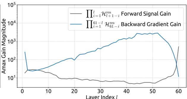
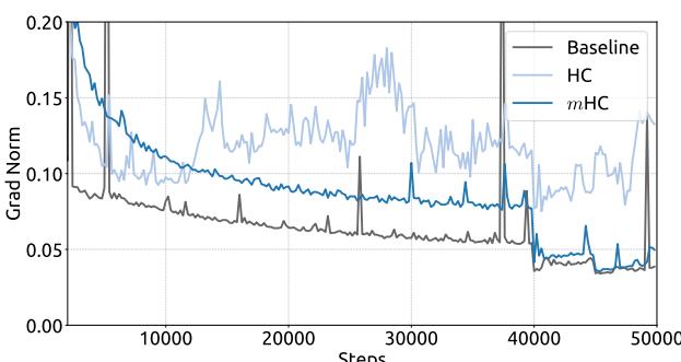
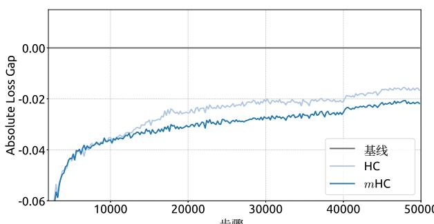
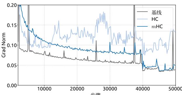
Figure 2 | Training Instability of Hyper-Connections (HC). This figure illustrates (a) the absolute loss gap of HC relative to mHC, and (b) the comparisons of gradient norms. All results are based on 27B models.
(b) Composite Mapping

3.2. System Overhead

While the computational complexity of HC remains manageable due to the linearity of the additional mappings, the system-level overhead prevents a non-negligible challenge. Specifically, memory access (I/O) costs often constitute one of the primary bottlenecks in modern model architectures, which is widely referred to as the “memory wall” (Dao et al., 2022). This bottleneck is frequently overlooked in architectural design, yet it decisively impacts runtime efficiency.

Focusing on the widely adopted pre-norm Transformer (Vaswani et al., 2017) architecture, we analyze the I/O patterns inherent to HC. Tab. 2 summarizes the per token memory access overhead in a single residual layer introduced by the $n$ -stream residual design. The analysis reveals that HC increases the memory access cost by a factor approximately proportional to $n$ . This excessive I/O demand significantly degrades training throughput without the mitigation of fused kernels. Besides, since ${\mathcal{H}}_l^{\mathrm{pre}}$ , ${\mathcal{H}}_l^{\mathrm{post}}$ , and ${\mathcal{H}}_l^{\mathrm{res}}$ involve learnable parameters, their intermediate activations are required for backpropagation. This results in a substantial increase in the GPU memory footprint, often necessitating gradient checkpointing to maintain feasible memory usage. Furthermore, HC requires $n$ -fold more communication cost in pipeline parallelism (Qi et al., 2024), leading to larger bubbles and decreasing the training throughput.

第007/19页（中文翻译）

(a) 绝对训练损失差距 vs. 训练步数

(b) 梯度范数 vs. 训练步数
图2|超连接（HC）的训练不稳定性。本图展示了（a）HC相对于改进型HC的绝对损失差距，以及（b）梯度范数的比较。所有结果均基于27B模型。

(a) 单层映射

(b) 复合映射
图3|超连接（HC）的传播不稳定性。本图展示了（a）单层映射 ${\mathrm{H}}_l^{\mathrm{res}}$ 和（b）复合映射 ${\prod }_{i=1}^{L-l}{\mathrm{H}}_{L-i}^{\mathrm{res}}$ 在27B模型内的传播动态。层索引 $l$ （x轴）将每个标准Transformer块展开为两个独立的层（注意力层和FFN层）。Amax增益幅度（y轴）计算为最大绝对行和（针对前向信号)与列和（针对反向梯度），并在选定序列的所有词元上取平均值。

3.2.系统开销

虽然超连接的计算复杂度由于额外映射的线性特性仍可管理，但系统级开销带来了不可忽视的挑战。具体而言，内存访问（I/O）成本通常是现代模型架构中的主要瓶颈之一，这被广泛称为“内存墙”（Dao等，2022）。这一瓶颈在架构设计中经常被忽视，但它对运行时效率具有决定性影响。

针对广泛采用的预归一化Transformer（Vaswani等，2017）架构，我们分析了HC固有的I/O模式。表2总结了由 $n$ 流残差设计在单个残差层中引入的每词元内存访问开销。分析表明，HC将内存访问成本增加了约与 $n$ 成正比的倍数。这种过度的I/O需求在没有融合内核缓解的情况下，会显著降低训练吞吐量。此外，由于 ${\mathrm{H}}_l^{\mathrm{pre}}$ 、H后和H残差涉及可学习参数，它们的中间激活在反向传播中是必需的。这导致GPU内存占用大幅增加，通常需要梯度检查点来维持可行的内存使用。再者，HC在流水线并行（Qi等，2024）中需要 $n$ 倍的通信开销，导致更大的气泡并降低训练吞吐量。

---

第008/19页（英文原文）

Table 2 | Comparison of Memory Access Costs Per Token. This analysis accounts for the overhead introduced by the residual stream maintenance in the forward pass, excluding the internal I/O of the layer function $\mathcal{F}$ .

Method	Operation	Read (Elements)	Write (Elements)
Residual Connection	Residual Merge	2C	C
	Total I/O	2C	C
Hyper-Connections	Calculate Hlpre, Hlpost, Hlres	nC	n2+2n
	Hlpre	nC+n	C
	Hlpost	C+n	nC
	Hlres	nC+n2	nC
	Residual Merge	2nC	nC
	Total I/O	(5n+1)C+n2+2n	(3n+1)C+n2+2n

4. Method

4.1. Manifold-Constrained Hyper-Connections

Drawing inspiration from the identity mapping principle (He et al., 2016b), the core premise of mHC is to constrain the residual mapping ${\mathcal{H}}_l^{\mathrm{res}}$ onto a specific manifold. While the original identity mapping ensures stability by enforcing ${\mathcal{H}}_l^{\mathrm{res}}=\mathbf{I}$ , it fundamentally precludes information exchange within the residual stream, which is critical for maximizing the potential of multi-stream architectures. Therefore, we propose projecting the residual mapping onto a manifold that simultaneously maintains the stability of signal propagation across layers and facilitates mutual interaction among residual streams to preserve the model’s expressivity. To this end, we restrict ${\mathcal{H}}_l^{\mathrm{res}}$ to be a doubly stochastic matrix, which has non-negative entries where both the rows and columns sum to 1. Formally, let ${\mathcal{M}}^{\mathrm{res}}$ denote the manifold of doubly stochastic matrices (also known as the Birkhoff polytope). We constrain ${\mathcal{H}}_l^{\mathrm{res}}$ to ${\mathcal{P}}_{{\mathcal{M}}^{\mathrm{res}}}({\mathcal{H}}_l^{\mathrm{res}})$ , defined as:

$${\mathcal{P}}_{{\mathcal{M}}^{\mathrm{res}}}({\mathcal{H}}_l^{\mathrm{res}}):=\left\{{\mathcal{H}}_l^{\mathrm{res}}\in {\mathbb{R}}^{n\times n}\mid {\mathcal{H}}_l^{\mathrm{res}}{1}_n=1_n,1_n^{\top }{\mathcal{H}}_l^{\mathrm{res}}=1_n^{\top },{\mathcal{H}}_l^{\mathrm{res}}⩾0\right\},\text{\hspace{1em}(6)}$$

where $1_n$ represents the $n$ -dimensional vector of all ones.

It is worth noting that when $n=1$ , the doubly stochastic condition degenerates to the scalar 1, thereby recovering the original identity mapping. The choice of double stochasticity confers several rigorous theoretical properties beneficial for large-scale model training:

1. Norm Preservation: The spectral norm of a doubly stochastic matrix is bounded by 1 (i.e., $\Vert {\mathcal{H}}_l^{\mathrm{res}}{\Vert }_2\le 1$ ). This implies that the learnable mapping is non-expansive, effectively mitigating the gradient explosion problem.
2. Compositional Closure: The set of doubly stochastic matrices is closed under matrix multiplication. This ensures that the composite residual mapping across multiple layers, ${\prod }_{i=1}^{L-l}{\mathcal{H}}_{L-i}^{\mathrm{res}}$ , remains doubly stochastic, thereby preserving stability throughout the entire depth of the model.
3. Geometric Interpretation via the Birkhoff Polytope: The set ${\mathcal{M}}^{\mathrm{res}}$ forms the Birkhoff polytope, which is the convex hull of the set of permutation matrices. This provides a clear geometric interpretation: the residual mapping acts as a convex combination of permutations. Mathematically, the repeated application of such matrices tends to increase

第008/19页（中文翻译）

表2|每个词元的内存访问开销对比。本分析考虑了前向传播中为维护残差流而引入的开销，不包括层函数F的内部I/O。

方法	手术	读取（元素数）	写入（元素数）
残差	残差合并	2C	C
连接	总输入输出	2C	C
超连接	计算 Hpre l, H后置 l, H残差 l	nC	n² + 2n
	H前 l	nC + n	C
	H后 l	C + n	nC
	H残差 l	nC + n²	nC
	残差合并	2nC	nC
	总输入输出	(5n + 1)C + n² + 2n	(3n + 1)C + n² + 2n

4. 方法

4.1.流形约束超连接

受恒等映射原理（He等，2016b）启发，mHC的核心前提是将残差映射 ${\mathrm{H}}_l^{\mathrm{res}}$ 约束到一个特定的流形上。虽然原始的恒等映射通过强制 ${\mathcal{H}}_l^{\mathrm{res}}=\mathbf{I}$ 来确保稳定性，但它从根本上阻止了残差流内部的信息交换，而这对于最大化多流架构的潜力至关重要。因此，我们建议将残差映射投影到一个流形上，该流形能同时维持信号跨层传播的稳定性，并促进残差流之间的相互交互，以保持模型的表达能力。为此，我们将 ${\mathrm{H}}_l^{\mathrm{res}}$ 限制为一个双随机矩阵，其元素非负且行和列的和均为1。形式化地，令 ${\mathrm{M}}^{\mathrm{res}}$ 表示双随机矩阵的流形（也称为Birkhoff多面体）。我们将 ${\mathrm{H}}_l^{\mathrm{res}}$ 约束为 ${\mathrm{P}}_{{\mathcal{M}}^{\mathrm{res}}}(\mathrm{H}$ 残差 $l)$ ，其定义为：

$${\mathcal{P}}_{{\mathcal{M}}^{\text{r e s}}}\left({\mathcal{H}}_l^{\text{r e s}}\right):=\left\{{\mathcal{H}}_l^{\text{r e s}}\in {\mathbb{R}}^{n\times n}\mid {\mathcal{H}}_l^{\text{r e s}}{1}_n=1_n,1_n^{\top }{\mathcal{H}}_l^{\text{r e s}}=1_n^{\top },{\mathcal{H}}_l^{\text{r e s}}⩾0\right\},\text{\hspace{1em}(6)}$$

其中 $1_n$ 表示所有元素为1的 $n$ 维向量。

值得注意的是，当 $n=1$ 时，双随机条件退化为标量 1，从而恢复了原始的恒等映射。选择双随机性赋予了几个严格的理论特性，有利于大规模模型训练：

1. 范数保持：双随机矩阵的谱范数以 1 为界 (i.e., $\Vert {\mathcal{H}}_l^{\mathrm{res}}{\Vert }_2\le 1$ )。这意味着可学习映射是非扩张的，能有效缓解梯度爆炸问题。
2. 组合封闭性：双随机矩阵的集合在矩阵乘法下是封闭的。这确保了跨越多层的复合残差映射，

${\prod }_{i=1}^{L-l}{\mathcal{H}}_{L-i}^{\mathrm{res}}$ ，仍然是双随机的，从而在整个模型的深度范围内保持稳定性。

3. 通过 Birkhoff 多面体进行几何解释：集合 ${\mathbf{M}}^{\mathrm{res}}$ 构成了 Birkhoff 多面体，它是置换矩阵集合的凸包。这提供了一个清晰的几何解释：残差映射的作用相当于置换的凸组合。从数学上讲，重复应用此类矩阵往往会增加

---

第009/19页（英文原文）

the mixing of information across streams monotonically, effectively functioning as a robust feature fusion mechanism.

Additionally, we impose non-negativity constraints on the input mappings ${\mathcal{H}}_l^{\mathrm{pre}}$ and output mappings ${\mathcal{H}}_l^{\mathrm{post}}$ . This constrain prevents signal cancellation arising from the composition of positive and negative coefficients, which can also be considered as a special manifold projection.

4.2. Parameterization and Manifold Projection

In this section, we detail the calculation process of ${\mathcal{H}}_l^{\mathrm{pre}},{\mathcal{H}}_l^{\mathrm{post}}$ , and ${\mathcal{H}}_l^{\mathrm{res}}$ in mHC. Given the input hidden matrix ${\mathbf{x}}_l\in {\mathbb{R}}^{n\times C}$ at the $l$ -th layer, we first flatten it into a vector ${\vec{\mathbf{x}}}_l=\mathrm{vec}({\mathbf{x}}_l)\in {\mathbb{R}}^{1\times nC}$ to preserve full context information. Then, we follow the original HC formulation to get the dynamic mappings and the static mappings as follows:

$$\{\begin{array}{l}{\vec{\mathbf{x}}}_l^{\prime }=\mathrm{RMSNorm}({\vec{\mathbf{x}}}_l)\\ {\tilde{\mathcal{H}}}_l^{\text{p r e}}={\alpha }_l^{\text{p r e}}\cdot \left({\vec{\mathbf{x}}}_l^{\prime }{\phi }_l^{\text{p r e}}\right)+{\mathbf{b}}_l^{\text{p r e}}\\ {\tilde{\mathcal{H}}}_l^{\text{p o s t}}={\alpha }_l^{\text{p o s t}}\cdot \left({\vec{\mathbf{x}}}_l^{\prime }{\phi }_l^{\text{p o s t}}\right)+{\mathbf{b}}_l^{\text{p o s t}}\\ {\tilde{\mathcal{H}}}_l^{\text{r e s}}={\alpha }_l^{\text{r e s}}\cdot \mathrm{mat}\left({\vec{\mathbf{x}}}_l^{\prime }{\phi }_l^{\text{r e s}}\right)+{\mathbf{b}}_l^{\text{r e s}},\end{array}\text{\hspace{1em}(7)}$$

where ${\phi }_l^{\mathrm{pre}},{\phi }_l^{\mathrm{post}}\in {\mathbb{R}}^{nC\times n}$ and ${\phi }_l^{\mathrm{res}}\in {\mathbb{R}}^{nC\times n^2}$ are linear projections for dynamic mappings and $\mathrm{mat}(\cdot )$ is a reshape function from ${\mathbb{R}}^{1\times n^2}$ to ${\mathbb{R}}^{n\times n}$ .

Then, the final constrained mappings are obtained via:

$$\{\begin{array}{l}{\mathcal{H}}_l^{\text{p r e}}=\sigma \left({\tilde{\mathcal{H}}}_l^{\text{p r e}}\right)\\ {\mathcal{H}}_l^{\text{p o s t}}=2\sigma \left({\tilde{\mathcal{H}}}_l^{\text{p o s t}}\right)\\ {\mathcal{H}}_l^{\text{r e s}}=Sinkhorn-Knopp\left({\tilde{\mathcal{H}}}_l^{\text{r e s}}\right),\end{array}\text{\hspace{1em}(8)}$$

where $\sigma (\cdot )$ denotes the Sigmoid function. The Sinkhorn-Knopp $(\cdot )$ operator firstly makes all elements to be positive via an exponent operator and then conducts iterative normalization process that alternately rescales rows and columns to sum to 1. Specifically, given a positive matrix ${\mathbf{M}}^{(0)}=\exp ({\tilde{\mathcal{H}}}_l^{\mathrm{res}})$ as the start point, the normalization iteration proceeds as:

$${\mathbf{M}}^{(t)}={\mathcal{T}}_r\left({\mathcal{T}}_c\left({\mathbf{M}}^{(t-1)}\right)\right),\text{\hspace{1em}(9)}$$

where ${\mathcal{T}}_r$ and ${\mathcal{T}}_c$ denote row and column normalization, respectively. This process converges to a doubly stochastic matrix ${\mathcal{H}}_l^{\mathrm{res}}={\mathbf{M}}^{(t_{\max })}$ as $t_{\max }\to \infty$ . We choose $t_{\max }=20$ as a practical value in our experiments.

4.3. Efficient Infrastructure Design

In this section, we detail the infrastructure design tailored for mHC. Through rigorous optimization, we implement mHC (with $n=4$ ) in large-scale models with a marginal training overhead of only $6.7\%$ .

4.3.1. Kernel Fusion

Observing that RMSNorm in $mHC$ imposes significant latency when operating on the high-dimensional hidden state ${\vec{\mathbf{x}}}_l\in {\mathbb{R}}^{1\times nC}$ , we reorder the dividing-by-norm operation to follow the

第009/19页（中文翻译）

信息在各流之间单调混合，有效地充当了稳健的特征融合机制。

此外，我们对输入映射 ${\mathcal{H}}_l^{\mathrm{pre}}$ 和输出映射 ${\mathcal{H}}_l^{\mathrm{post}}$ 施加了非负性约束。这一约束可以防止由正负系数组合引起的信号抵消，这也可以被视为一种特殊的流形投影。

4.2.参数化与流形投影

在本节中，我们将详细阐述 $m$ 超连接中 ${\mathcal{H}}_l^{\mathrm{pre}}{\mathcal{H}}_l^{\mathrm{post}}$ 、 ${\mathcal{H}}_l^{\mathrm{res}}$ 的计算过程。给定第 $l$ 层的输入隐层矩阵 ${\mathbf{x}}_l\in {\mathbb{R}}^{n\times C}$ ，我们首先将其展平为向量 ${\vec{\mathbf{x}}}_l=\mathrm{vec}({\mathbf{x}}_l)\in {\mathbb{R}}^{1\times nC}$ 以保留完整的上下文信息。然后，我们遵循原始超连接公式，得到动态映射和静态映射如下：

$$\{\begin{array}{l}{\vec{\mathbf{x}}}_l^{\prime }=\mathrm{RMSNorm}({\vec{\mathbf{x}}}_l)\\ {\tilde{\mathcal{H}}}_l^{\text{p r e}}={\alpha }_l^{\text{p r e}}\cdot \left({\vec{\mathbf{x}}}_l^{\prime }{\phi }_l^{\text{p r e}}\right)+{\mathbf{b}}_l^{\text{p r e}}\\ {\tilde{\mathcal{H}}}_l^{\text{p o s t}}={\alpha }_l^{\text{p o s t}}\cdot \left({\vec{\mathbf{x}}}_l^{\prime }{\phi }_l^{\text{p o s t}}\right)+{\mathbf{b}}_l^{\text{p o s t}}\\ {\tilde{\mathcal{H}}}_l^{\text{r e s}}={\alpha }_l^{\text{r e s}}\cdot \mathrm{mat}\left({\vec{\mathbf{x}}}_l^{\prime }{\phi }_l^{\text{r e s}}\right)+{\mathbf{b}}_l^{\text{r e s}},\end{array}\text{\hspace{1em}(7)}$$

其中 ${\phi }_l^{\mathrm{pre}}{\phi }_l^{\mathrm{post}}\in {\mathbb{R}}^{nC\times n}$ 和 ${\phi }_l^{\mathrm{res}}\in {\mathbb{R}}^{nC\times n^2}$ 是用于动态映射的线性投影，而mat(·）是一个从 ${\mathbb{R}}^{1\times n^2}$ 重塑到 ${\mathbb{R}}^{n\times n}$ 的重塑函数。

随后，通过以下方式获得最终的约束映射：

$$\{\begin{array}{l}{\mathcal{H}}_l^{\text{p r e}}=\sigma \left({\tilde{\mathcal{H}}}_l^{\text{p r e}}\right)\\ {\mathcal{H}}_l^{\text{p o s t}}=2\sigma \left({\tilde{\mathcal{H}}}_l^{\text{p o s t}}\right)\\ {\mathcal{H}}_l^{\text{r e s}}=Sinkhorn-Knopp\left({\tilde{\mathcal{H}}}_l^{\text{r e s}}\right),\end{array}\text{\hspace{1em}(8)}$$

其中 $\sigma (\cdot )$ 表示Sigmoid函数。Sinkhorn-Knopp( $\cdot$ ) 算子首先通过指数算子使所有元素为正,然后进行迭代归一化过程, 交替重新缩放行和列使其和为1。具体而言, 给定一个正矩阵 ${\mathbf{M}}^{(0)}=\exp ({\tilde{\mathcal{H}}}_l^{\mathrm{res}})$ 作为起点, 归一化迭代过程如下:

$${\mathbf{M}}^{(t)}={\mathcal{T}}_r\left({\mathcal{T}}_c\left({\mathbf{M}}^{(t-1)}\right)\right),\text{\hspace{1em}(9)}$$

其中 ${\mathrm{T}}_r$ 和 ${\mathrm{T}}_c$ 分别表示行归一化和列归一化。此过程收敛于一个双随机矩阵 ${\mathrm{H}}_l^{\mathrm{res}}={\mathbf{M}}^{(t_{\max })}$ 当 $t_{\max }\to \infty$ 。在我们的实验中，我们选择 $t_{\max }=20$ 作为一个实际值。

4.3.高效基础设施设计

在本节中，我们将详细介绍为mHC量身定制的基础设施设计。通过严格的优化，我们在大规模模型中实现了mHC（使用 $n=4$ ），其边际训练开销仅为 $6.7\%$ 。

4.3.1. 核融合

我们观察到，mHC中的RMSNorm在对高维隐藏状态 ${\vec{\mathbf{x}}}_l\in {\mathbb{R}}^{1\times nC}$ 进行手术时会造成显著的延迟，因此我们重新安排除以范数的操作，使其跟随

---

第010/19页（英文原文）

matrix multiplication. This optimization maintains mathematical equivalence while improving efficiency. Furthermore, we employ mixed-precision strategies to maximize numerical accuracy without compromising speed, and fuse multiple operations with shared memory access into unified compute kernels to reduce memory bandwidth bottlenecks. Based on the inputs and parameters detailed in Eq. (10) to (13), we implement three specialized mHC kernels to compute ${\mathcal{H}}_l^{\mathrm{pre}}$ , ${\mathcal{H}}_l^{\mathrm{post}}$ , and ${\mathcal{H}}_l^{\mathrm{res}}$ . In these kernels, the biases and linear projections are consolidated into ${\mathbf{b}}_l$ and ${\phi }_l$ , and the RMSNorm weight is also absorbed in ${\phi }_l$ .

• Eq. (14) to (15): We develop a unified kernel that fuses two scans on ${\vec{\mathbf{x}}}_l$ , leveraging matrix multiplication units to maximize memory bandwidth utilization. The backward pass—comprising two matrix multiplications—is similarly consolidated into a single kernel, eliminating redundant reloading of ${\vec{\mathbf{x}}}_l$ . Both kernels feature a finely tuned pipeline (load, cast, compute, store) to efficiently handle mixed-precision processing.
• Eq. (16) to (18): These lightweight operations on small coefficients are opportunistically fused into a single kernel, significantly reducing kernel launch overhead.
• Eq. (19): We implement the Sinkhorn-Knopp iteration within a single kernel. For the backward pass, we derive a custom backward kernel that recomputes the intermediate results on-chip and traverses the entire iteration.

$${\phi }_l:\text{t f l o a t}32[nC,n^2+2n]\text{\hspace{1em}(10)}$$

$${\vec{\mathbf{x}}}_l:\text{b f l o a t}16[1,nC]\text{\hspace{1em}(11)}$$

$${\alpha }_l^{\text{p r e}},{\alpha }_l^{\text{p o s t}},{\alpha }_l^{\text{r e s}}:\text{f l o a t 3 2}\text{S c a l a r s}\text{\hspace{1em}(12)}$$

$${\mathbf{b}}_l:\text{f l o a t 3 2}[1,n^2+2n]\text{\hspace{1em}(13)}$$

$$\begin{array}{l}\left[{\tilde{\mathcal{H}}}_l^{\text{p r e}},{\tilde{\mathcal{H}}}_l^{\text{p o s t}},{\tilde{\mathcal{H}}}_l^{\text{r e s}}\right]:\text{f l o a t 3 2}={\vec{\mathrm{x}}}_l{\phi }_l(14)\\ r:\text{f l o a t 3 2}={\Vert {\vec{\mathbf{x}}}_l\Vert }_2/\sqrt{nC}(15)\end{array}$$

$$\begin{array}{l}\left[{\tilde{\mathcal{H}}}_l^{\text{p r e}},{\tilde{\mathcal{H}}}_l^{\text{p o s t}},{\tilde{\mathcal{H}}}_l^{\text{r e s}}\right]:\text{f l o a t 3 2}=1/r\left[{\alpha }_l^{\text{p r e}}{\tilde{\mathcal{H}}}_l^{\text{p r e}},{\alpha }_l^{\text{p o s t}}{\tilde{\mathcal{H}}}_l^{\text{p o s t}},{\alpha }_l^{\text{r e s}}{\tilde{\mathcal{H}}}_l^{\text{r e s}}\right]+{\mathbf{b}}_l(16)\\ {\mathcal{H}}_l^{\text{p r e}}:\text{f l o a t 3 2}=\sigma \left({\tilde{\mathcal{H}}}_l^{\text{p r e}}\right)(17)\\ {\mathcal{H}}_l^{\text{p o s t}}:\text{f l o a t 3 2}=2\sigma \left({\tilde{\mathcal{H}}}_l^{\text{p o s t}}\right)(18)\\ {\mathcal{H}}_l^{\text{r e s}}:\text{f l o a t 3 2}=\text{S i n k h o r n - K n o p p}\left({\tilde{\mathcal{H}}}_l^{\text{r e s}}\right)(19)\end{array}$$

Using the coefficients derived from the aforementioned kernels, we introduce two additional kernels to apply these mappings: one for ${\mathcal{F}}_{\mathrm{pre}}:={\mathcal{H}}_l^{\mathrm{pre}}{\mathbf{x}}_l$ and another for ${\mathcal{F}}_{\mathrm{post},\mathrm{res}}:={\mathcal{H}}_l^{\mathrm{res}}{\mathbf{x}}_l+{\mathcal{H}}_l^{\mathrm{post}}\mathcal{F}(\cdot ,\cdot )$ . Through fusing the application of ${\mathcal{H}}_l^{\mathrm{post}}$ and ${\mathcal{H}}_l^{\mathrm{res}}$ with residual merging, we reduce the number of elements read from $(3n+1)C$ to $(n+1)C$ and the number of elements written from $3nC$ to $nC$ for this kernel. We efficiently implement the majority of kernels (excluding Eq. (14) to (15)) using TileLang (Wang et al., 2025). This framework streamlines the implementation of kernels with complex calculation process and allows us to fully utilize the memory bandwidth with minimal engineering effort.

4.3.2. Recomputing

The $n$ -stream residual design introduces substantial memory overhead during training. To mitigate this, we discard the intermediate activations of the mHC kernels after the forward pass and recompute them on-the-fly in the backward pass, through re-executing the mHC kernels

第010/19页（中文翻译）

矩阵乘法。这项优化在保持数学等价性的同时提高了效率。此外，我们采用混合精度策略，在不牺牲速度的前提下最大化数值精度，并将多个具有共享内存访问的操作融合为统一的计算内核，以减少内存带宽瓶颈。基于公式(10)至(13)中详述的输入和参数，我们实现了三个专门的mHC内核，用于计算H pre $l$ 、 ${\mathrm{H}}_l^{\mathrm{post}}$ 和H res $l$ 。在这些内核中，偏置和线性投影被合并到 ${\mathbf{b}}_l$ 和 ${\phi }_l$ 中，RMSNorm权重也被吸收到 ${\phi }_l$ 中。

• 公式(14)至(15): 我们开发了一个统一的内核, 融合了对 ${\vec{\mathbf{x}}}_l$ 的两次扫描, 利用矩阵乘法单元以最大化内存带宽利用率。反向传播——包含两次矩阵乘法——同样被整合到单个内核中,消除了 ${\vec{\mathbf{x}}}_l$ 的冗余重新加载。两个内核都采用精细调优的流水线（加载、转换、计算、存储）,以高效处理混合精度处理。
• 公式(16)至(18)：这些针对小系数的轻量级操作被适时地融合到单个内核中，显著减少了内核启动开销。
• 公式(19)：我们在单个内核内实现了Sinkhorn-Knopp迭代。对于反向传播，我们推导了一个自定义的反向内核，该内核在片上重计算中间结果并遍历整个迭代过程。

$${\phi }_l:\text{t f l o a t}32[nC,n^2+2n]\text{\hspace{1em}(10)}$$

$${\vec{\mathbf{x}}}_l:\text{b f l o a t}16[1,nC]\text{\hspace{1em}(11)}$$

$${\alpha }_l^{\text{p r e}},{\alpha }_l^{\text{p o s t}},{\alpha }_l^{\text{r e s}}:\text{f l o a t 3 2}\text{S c a l a r s}\text{\hspace{1em}(12)}$$

$${\mathbf{b}}_l:\text{f l o a t 3 2}[1,n^2+2n]\text{\hspace{1em}(13)}$$

$$\begin{array}{l}\left[{\tilde{\mathcal{H}}}_l^{\text{p r e}},{\tilde{\mathcal{H}}}_l^{\text{p o s t}},{\tilde{\mathcal{H}}}_l^{\text{r e s}}\right]:\text{f l o a t 3 2}={\vec{\mathbf{x}}}_l{\phi }_l(14)\\ r:\text{f l o a t 3 2}={\Vert {\vec{\mathbf{x}}}_l\Vert }_2/\sqrt{nC}(15)\end{array}$$

$$\begin{array}{l}\left[{\tilde{\mathcal{H}}}_l^{\mathrm{pre}},{\tilde{\mathcal{H}}}_l^{\mathrm{post}},{\tilde{\mathcal{H}}}_l^{\mathrm{res}}\right]:\text{f l o a t 3 2}=1/r\left[{\alpha }_l^{\mathrm{pre}}{\tilde{\mathcal{H}}}_l^{\mathrm{pre}},{\alpha }_l^{\mathrm{post}}{\tilde{\mathcal{H}}}_l^{\mathrm{post}},{\alpha }_l^{\mathrm{res}}{\tilde{\mathcal{H}}}_l^{\mathrm{res}}\right]+{\mathbf{b}}_l(16)\\ {\mathcal{H}}_l^{\text{p r e}}:\text{f l o a t 3 2}=\sigma \left({\tilde{\mathcal{H}}}_l^{\text{p r e}}\right)(17)\\ {\mathcal{H}}_l^{\text{p o s t}}:\text{f l o a t 3 2}=2\sigma \left({\tilde{\mathcal{H}}}_l^{\text{p o s t}}\right)(18)\\ {\mathcal{H}}_l^{\text{r e s}}:\text{f l o a t 3 2}=\text{S i n k h o r n - K n o p p}\left({\tilde{\mathcal{H}}}_l^{\text{r e s}}\right)(19)\end{array}$$

利用从上述内核推导出的系数，我们引入了两个额外的内核来应用这些映射：一个用于 ${\mathcal{F}}_{\mathrm{pre}}:={\mathcal{H}}_l^{\mathrm{pre}}{\mathbf{x}}_l$ ，另一个用于 ${\mathcal{F}}_{\mathrm{post}\mathrm{res}}:={\mathcal{H}}_l^{\mathrm{res}}{\mathbf{x}}_l+{\mathcal{H}}_l^{{\mathrm{post}}^{\top }}\mathcal{F}(\cdot ,\cdot )$ 。通过将 ${\mathcal{H}}_l^{\mathrm{post}}$ 和 ${\mathcal{H}}_l^{\mathrm{res}}$ 的应用与残差合并相融合，我们将该内核需要从 $(3n+1)C$ 读取的元素数量减少到 $(n+1)C$ ，并将需要写入的元素数量从 $3nC$ 减少到 $nC$ 。我们高效地实现了大部分内核（不包括公式(14)至(15)），使用的是TileLang（Wang等人，2025）。该框架简化了具有复杂计算过程的内核实现，并使我们能够以最小的工程努力充分利用内存带宽。

4.3.2. 重计算

$n$ 流残差设计在训练期间引入了显著的内存开销。为了缓解这一问题，我们在前向传播后丢弃 $m$ 超连接核的中间激活，并在反向传播中通过重新执行 $m$ 超连接核来即时重计算它们。

---

第011/19页（英文原文）

without the heavy layer function $\mathcal{F}$ . Consequently, for a block of $L_r$ consecutive layers, we need only store the input ${\mathbf{x}}_{l_0}$ to the first layer. Excluding lightweight coefficients while accounting for the pre-norm with in $\mathcal{F}$ , Tab. 3 summarizes the intermediate activations preserved for the backward pass.

Table 3 | Stored and Recomputed Intermediate Activations We list per token activation preserved for the backward pass and the transient activation recomputed in $L_r$ consecutive layers. Layer $l_0$ represents the first layer in $L_r$ layers and layer $l$ is in $[l_0,l_0+L_r-1]$ .

Activations	x l0	F(Hl pre x l, Wl)	x l	Hl pre x l	RMSNorm(Hl pre x l)
Size (Elements)	nC	C	nC	C	C
Stored Method	Every Lr layers	Every layer	Transient inside Lr layers

Since mHC kernels recomputation is performed for blocks of $L_r$ consecutive layers, given a total of $L$ layers, we must persistently store the first layer input ${\mathbf{x}}_{l_0}$ for all $\lceil \frac{L}{L_r}\rceil$ blocks for the backward pass. In addition to this resident memory, the recomputation process introduces a transient memory overhead of $(n+2)C\times L_r$ elements for the active block, which determines the peak memory usage during backpropagation. Consequently, we determine the optimal block size $L_r^{\ast }$ by minimizing the total memory footprint corresponded to $L_r$ :

$$L_r^{\ast }=\arg \underset{L_r}{\min }\left[nC\times \lceil \frac{L}{L_r}\rceil +(n+2)C\times L_r\right]\approx \sqrt{\frac{nL}{n+2}}.\text{\hspace{1em}(20)}$$

Furthermore, pipeline parallelism in large-scale training imposes a constraint: recomputation blocks must not cross pipeline stage boundaries. Observing that the theoretical optimum $L_r^{\ast }$ typically aligns with the number of layers per pipeline stage, we choose to synchronize the recomputation boundaries with the pipeline stages.

4.3.3. Overlapping Communication in DualPipe

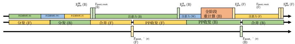
In large-scale training, pipeline parallelism is the standard practice for mitigating parameter and gradient memory footprints. Specifically, we adopt the DualPipe schedule (Liu et al., 2024b), which effectively overlaps scale-out interconnected communication traffic, such as those in expert and pipeline parallelism. However, compared to the single-stream design, the proposed $n$ -stream residual in mHC incurs substantial communication latency across pipeline stages. Furthermore, at stage boundaries, the recomputation of mHC kernels for all $L_r$ layers introduces non-negligible computational overhead. To address these bottlenecks, we extend the DualPipe schedule (see Fig. 4) to facilitate improved overlapping of communication and computation at pipeline stage boundaries.

Notably, to prevent blocking the communication stream, we execute the ${\mathcal{F}}_{\mathrm{post},\mathrm{res}}$ kernels of MLP (i.e. FFN) layers on a dedicated high-priority compute stream. We further refrain from employing persistent kernels for long-running operations in attention layers, thereby preventing extended stalls. This design enables the preemption of overlapped attention computations, allowing for flexible scheduling while maintaining high utilization of the compute device’s processing units. Furthermore, the recomputation process is decoupled from pipeline communication dependencies, as the initial activation of each stage ${\mathbf{x}}_{l_0}$ is already cached locally.

第011/19页（中文翻译）

无需繁重的层函数F。因此，对于连续 $L_r$ 个层的区块，我们仅需存储第一层的输入 ${\mathbf{x}}^{l_0}$ 。在排除轻量级系数并考虑F中的预归一化后，表3总结了为反向传播保留的中间激活。

表 3 | 存储与重计算的中间激活我们列出了为反向传播保存的每个词元激活以及在 $L_r$ 个连续层中重计算的瞬时激活。层 $l_0$ 表示 $L_r$ 层中的第一层，层 $l$ 位于 $[l_0,l_0+L_r-1]$ 。

激活	x l0	F (Hl pre x l, Wl)	x l	H pre l x l RMSNorm(Hl pre l x)
大小（元素数）	nC	C	nC	C	C
存储方法	每Lr层	每一层		Lr层内的临时开销

由于 $m$ 超连接内核重计算是针对 $L_r$ 个连续层组成的块执行的，给定总共有 $L$ 层，我们必须为所有 $\lceil \frac{L}{L_r}\rceil$ 个块持久存储第一个层的输入 $\mathbf{x}{l}_0$ 以供反向传播使用。除了这部分常驻内存外，重计算过程还会为活动块引入 $(n+2)C\times L_r$ 个元素的临时内存开销，这决定了反向传播期间的峰值内存使用量。因此，我们通过最小化对应于 $L_r$ 的总内存占用来确定最优块大小 $L_r^{\ast }$ ：

$$L_r^{\ast }=\arg \underset{L_r}{\min }\left[nC\times \lceil \frac{L}{L_r}\rceil +(n+2)C\times L_r\right]\approx \sqrt{\frac{nL}{n+2}}.\text{\hspace{1em}(20)}$$

此外，大规模训练中的流水线并行施加了一个约束：重计算块不得跨越流水线阶段边界。鉴于理论最优值 $L_r^{\ast }$ 通常与每个流水线阶段的层数一致，我们选择将重计算边界与流水线阶段同步。

4.3.3. DualPipe 中的通信重叠

在大规模训练中，流水线并行是减轻参数和梯度内存占用的标准做法。具体而言，我们采用了 DualPipe 调度（Liu 等, 2024b），它能有效重叠横向扩展互连通信流量，例如专家并行和流水线并行中的流量。然而，与单流设计相比，mHC 中提出的 $n$ 流残差在流水线阶段之间产生了显著的通信延迟。此外，在流水线阶段边界处，为所有 $L_r$ 层重新计算 mHC 内核会带来不可忽略的计算开销。为了解决这些瓶颈，我们扩展了 DualPipe 调度（见图 4），以促进在流水线阶段边界处更好地重叠通信与计算。

值得注意的是，为了防止阻塞通信流，我们在一个专用的高优先级计算流上执行MLP（即FFN）层的 ${\mathcal{F}}_{\mathrm{postres}}$ 内核。我们进一步避免在注意力层中对长时间运行的操作使用持久内核，从而防止长时间的停滞。这种设计使得重叠的注意力计算可以被抢占，从而在保持计算设备处理单元高利用率的同时，实现灵活的调度。此外，重计算过程与流水线通信依赖解耦，因为每个阶段的初始激活 $x{l}_0$ 已缓存在本地。

---

第012/19页（英文原文）

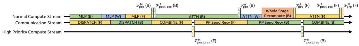
Figure 4 | Communication-Computation Overlapping for mHC. We extend the DualPipe schedule to handle the overhead introduced by mHC. Lengths of each block are illustrative only and do not represent actual duration. (F), (B), (W) refers to forward pass, backward pass, weight gradient computation, respectively. ${\mathcal{F}}^{\mathrm{A}}$ and ${\mathcal{F}}^{\mathrm{M}}$ represents kernels corresponded to Attention and MLP, respectively.

5. Experiments

5.1. Experimental Setup

We validate the proposed method via language model pre-training, conducting a comparative analysis between the baseline, HC, and our proposed mHC. Utilizing MoE architectures inspired by DeepSeek-V3 (Liu et al., 2024b), we train four distinct model variants to cover different evaluation regimes. Specifically, the expansion rate $n$ for both HC and mHC is set to 4. Our primary focus is a 27B model trained with a dataset size proportional to its parameters, which serves as the subject for our system-level main results. Expanding on this, we analyze the compute scaling behavior by incorporating smaller 3B and 9B models trained with proportional data, which allows us to observe performance trends across varying compute. Additionally, to specifically investigate the token scaling behavior, we train a separate 3B model on a fixed corpus of 1 trillion tokens. Detailed model configurations and training hyper-parameters are provided in Appendix A.1.

5.2. Main Results

(a) Absolute Training Loss Gap vs. Training Steps

(b) Gradient Norm vs. Training Steps
Figure 5 | Training Stability of Manifold-Constrained Hyper-Connections (mHC). This figure illustrates (a) the absolute training loss gap of mHC and HC relative to the baseline, and (b) the gradient norm of the three methods. All experiments utilize the 27B model. The results demonstrate that mHC exhibits improved stability in terms of both loss and gradient norm.

We begin by examining the training stability and convergence of the 27B models. As illustrated in Fig. 5 (a), mHC effectively mitigates the training instability observed in HC, achieving a final loss reduction of 0.021 compared to the baseline. This improved stability is further corroborated by the gradient norm analysis in Fig. 5 (b), where mHC exhibits significantly better behavior than HC, maintaining a stable profile comparable to the baseline.

第012/19页（中文翻译）

图4|流形约束超连接的mHC通信-计算重叠。我们扩展了DualPipe调度以处理mHC引入的开销。每个区块的长度仅为示意，不代表实际持续时间。(F)、(B)、(W)分别指代前向传播、反向传播、权重梯度计算。 ${\mathbf{F}}^{\mathrm{A}}$ 和 $\mathbf{FM}$ 分别代表对应于注意力与多层感知机的内核。

5. 实验

5.1. 实验设置

我们通过语言模型预训练来验证所提出的方法，并对基线、HC和我们提出的 $m\mathrm{HC}$ 进行对比分析。利用受DeepSeek-V3(Liu等,2024b)启发的MoE架构，我们训练了四个不同的模型变体，以覆盖不同的评估范围。具体来说，HC和 $m\mathrm{HC}$ 的扩展率 $n$ 均设置为4。我们的主要关注点是一个27B模型，其训练数据集规模与其参数成正比，这构成了我们系统级主要结果的研究对象。在此基础上，我们通过纳入按比例数据训练的较小的3B模型和9B模型来分析计算扩展行为，这使我们能够观察不同计算量下的性能趋势。此外，为了专门研究代币扩展行为，我们在一个固定的1万亿代币语料库上训练了一个单独的3B模型。详细的模型配置和训练超参数在附录A.1中提供。

5.2.主要结果

(a) 绝对训练损失差距 vs. 训练步数

(b) 梯度范数 vs. 训练步数
图5|流形约束超连接(mHC)的训练稳定性。本图展示了(a)mHC和HC相对于基线的绝对训练损失差距，以及(b)三种方法的梯度范数。所有实验均使用27B模型。结果表明，mHC在损失和梯度范数方面均表现出更高的稳定性。

我们首先考察27B模型的训练稳定性和收敛情况。如图5(a)所示，mHC有效缓解了在HC中观察到的训练不稳定，与基线相比实现了0.021的最终损失降低。这种改善的稳定性在图5(b)的梯度范数分析中得到了进一步证实，其中mHC表现出比HC显著更好的行为，保持了与基线相当的稳定态势。

---

第013/19页（英文原文）

Table 4 | System-level Benchmark Results for 27B Models. This table compares the zero-shot and few-shot performance of the Baseline, HC, and mHC across 8 diverse downstream benchmarks. mHC consistently outperforms the Baseline and surpasses HC on the majority of benchmarks, demonstrating its effectiveness in large-scale pre-training.

Benchmark (Metric)	BBH (EM)	DROP (F1)	GSM8K (EM)	HellaSwag (Acc.)	MATH (EM)	MMLU (Acc.)	PIQA (Acc.)	TriviaQA (EM)
# Shots	3-shot	3-shot	8-shot	10-shot	4-shot	5-shot	0-shot	5-shot
27B Baseline	43.8	47.0	46.7	73.7	22.0	59.0	78.5	54.3
27B w/ HC	48.9	51.6	53.2	74.3	26.4	63.0	79.9	56.3
27B w/ mHC	51.0	53.9	53.8	74.7	26.0	63.4	80.5	57.6

Tab. 4 presents the downstream performance across a diverse set of benchmarks (Bisk et al., 2020; Cobbe et al., 2021; Hendrycks et al., 2020, 2021; Joshi et al., 2017; Zellers et al., 2019). mHC yields comprehensive improvements, consistently outperforming the baseline and surpassing HC on the majority of tasks. Notably, compared to HC, mHC further enhances the model’s reasoning capabilities, delivering performance gains of $2.1\%$ on BBH (Suzgun et al., 2022) and $2.3\%$ on DROP (Dua et al., 2019).

5.3. Scaling Experiments

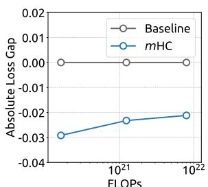
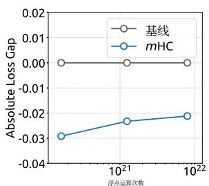
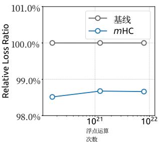
(a) Compute Scaling Curve

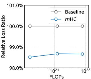
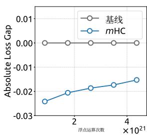
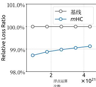
Figure 6 | Scaling properties of mHC compared to the Baseline. (a) Compute Scaling Curve. Solid lines depict the performance gap across different compute budgets. Each point represents a specific compute-optimal configuration of model size and dataset size, scaling from 3B and 9B to 27B parameters. (b) Token Scaling Curve. Trajectory of the 3B model during training. Each point represents the model’s performance at different training tokens. Detailed architectures and training configurations are provided in Appendix A.1.

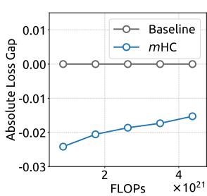
(b) Token Scaling Curve

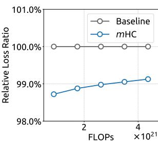
To assess the scalability of our approach, we report the relative loss improvement of mHC against the baseline across different scales. In Fig. 6 (a), we plot the compute scaling curve spanning 3B, 9B, and 27B parameters. The trajectory indicates that the performance advantage is robustly maintained even at higher computational budgets, showing only marginal attenuation. Furthermore, we examine the within-run dynamics in Fig. 6 (b), which presents the token scaling curve for the 3B model. Collectively, these findings validate the effectiveness of mHC in large-scale scenarios. This conclusion is further corroborated by our in-house large-scale training experiments.

第013/19页（中文翻译）

表4|27B模型的系统级基准结果。本表比较了基线、HC和mHC在8个不同下游基准上的零样本和少样本性能。mHC始终优于基线，并在大多数基准上超越了HC，证明了其在大规模预训练中的有效性。

基准 (指标)	BBH (EM)	DROP (F1)	GSM8K (EM)	HellaSwag (准确率)	MATH (EM)	MMLU (准确率)	PIQA (准确率)	TriviaQA (EM)
#示例数	3示例	3示例	8示例	10示例	4示例	5示例	零示例	5示例
27B基线	43.8	47.0	46.7	73.7	22.0	59.0	78.5	54.3
27B带HC	48.9	51.6	53.2	74.3	26.4	63.0	79.9	56.3
27B带mHC	51.0	53.9	53.8	74.7	26.0	63.4	80.5	57.6

表4展示了在多样化基准测试集（Bisk等，2020；Cobbe等，2021；Hendrycks等，2020，2021；Joshi等，2017；Zellers等，2019）上的下游性能。mHC带来了全面的改进，始终优于基线，并在大多数任务上超越了HC。值得注意的是，与HC相比，mHC进一步增强了模型的推理能力，在BBH（Suzgun等，2022）上实现了 $2.1\%$ 的性能提升，在DROP（Dua等，2019）上实现了 $2.3\%$ 的性能提升。

5.3.扩展实验

(a) 计算扩展曲线

(b) 代币扩展曲线
图6|mHC与基线的扩展特性对比。(a)计算扩展曲线。实线描绘了不同计算预算下的性能差距。每个点代表一个特定的计算最优配置，包括模型规模和数据集规模，参数规模从3B和9B扩展到27B。(b)代币扩展曲线。展示了3B模型在训练过程中的轨迹。每个点代表模型在不同训练词元数量下的性能。详细的架构和训练配置见附录A.1。

为评估我们方法的可扩展性，我们报告了mHC相对于基线在不同规模下的相对损失改进。在图6(a)中，我们绘制了涵盖3B、9B和27B参数的计算扩展曲线。其轨迹表明，即使在更高的计算预算下，性能优势也能稳健保持，仅出现边际衰减。此外，我们在图6(b)中检查了运行内的动态变化，该图展示了3B模型的代币扩展曲线。总的来说，这些发现验证了mHC在大规模场景中的有效性。这一结论在我们的内部大规模训练实验中得到了进一步证实。

---

第014/19页（英文原文）

(a) Single-Layer Mapping

(b) Composite Mapping

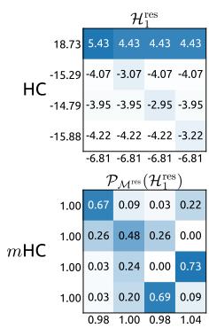
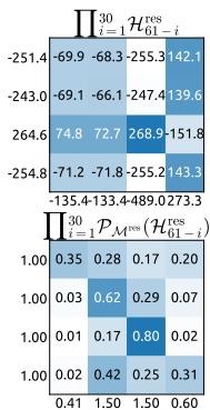
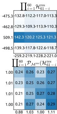
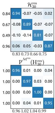
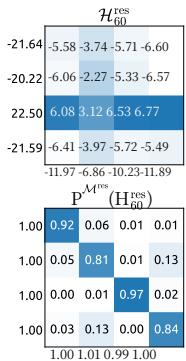
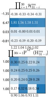
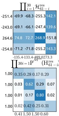
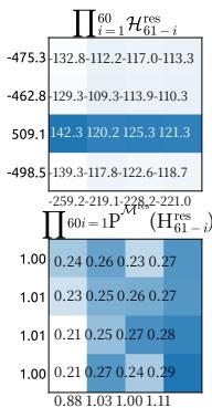
Figure 8 | Visualizations of Learnable Mappings. This figure displays representative single-layer and composite mappings for HC (first row) and mHC (second row). Each matrix is computed by averaging over all tokens within a selected sequence. The labels annotated along the y-axis and x-axis indicate the forward signal gain (row sum) and the backward gradient gain (column sum), respectively.

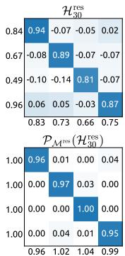
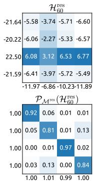
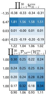
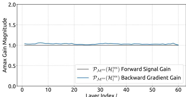
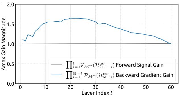
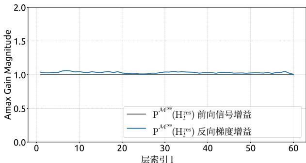
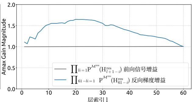
Figure 7 | Propagation Stability of Manifold-Constrained Hyper-Connections (mHC). This figure illustrates the propagation dynamics of (a) the single-layer mapping ${\mathcal{P}}_{{\mathcal{M}}^{\mathrm{res}}}({\mathcal{H}}_l^{\mathrm{res}})$ and (b) the composite mapping ${\prod }_{i=1}^{L-l}{\mathcal{P}}_{{\mathcal{M}}^{\mathrm{res}}}({\mathcal{H}}_{L-i}^{\mathrm{res}})$ within the 27B model. The results demonstrate that mHC significantly enhances propagation stability compared to HC.

5.4. Stability Analysis

Similar to Fig. 3, Fig. 7 illustrates the propagation stability of mHC. Ideally, the single-layer mapping satisfies the doubly stochastic constraint, implying that both the forward signal gain and the backward gradient gain should equal to 1. However, practice implementations utilizing the Sinkhorn-Knopp algorithm must limit the number of iterations to achieve computational efficiency. In our settings, we use 20 iterations to obtain an approximate solution. Consequently, as shown in Fig. 7(a), the backward gradient gain deviates slightly from 1. In the composite case shown in Fig. 7(b), the deviation increases but remains bounded, reaching a maximum value of approximately 1.6. Notably, compared to the maximum gain magnitude of nearly 3000 in HC, mHC significantly reduces it by three orders of magnitude. These results demonstrate that mHC significantly enhances propagation stability compared to HC, ensuring stable forward signal and backward gradient flows. Additionally, Fig. 8 displays representative mappings. We observe that for HC, when the maximum gain is large, other values also tend to be significant, which indicates general instability across all propagation paths. In contrast, mHC consistently yields stable results.

第014/19页（中文翻译）

(a) 单层映射

(b) 复合映射
图7|流形约束超连接的传播稳定性(mHC)。本图展示了(a)单层映射 ${\mathrm{P}}_{{\mathcal{M}}^{\mathrm{res}}}\left({\mathrm{H}}_l^{\mathrm{res}}\right)$ 和(b)复合映射 ${\prod }_{i=1}^{L-l}{\mathcal{P}}_{{\mathcal{M}}^{\mathrm{res}}}\left({\mathcal{H}}_{L-l}^{\mathrm{res}}\right)$ 在27B模型中的传播动态。结果表明，mHC相比HC显著增强了传播稳定性。

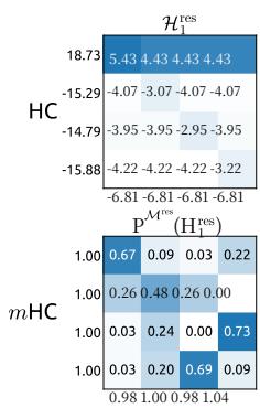
图8|可学习映射可视化。本图展示了HC（第一行）和mHC（第二行）的代表性单层映射与复合映射。每个矩阵通过对选定序列内所有词元取平均计算得出。y轴和x轴上的标注标签分别表示前向信号增益（行和）与反向梯度增益（列和）。

5.4. 稳定性分析

与图3类似，图7展示了mHC的传播稳定性。理想情况下，单层映射应满足双随机约束，这意味着前向信号增益和反向梯度增益都应等于1。然而，实践中使用Sinkhorn-Knopp算法的实现必须限制迭代次数以实现计算效率。在我们的设置中，我们使用20次迭代来获得近似解。因此，如图7(a)所示，反向梯度增益会略微偏离1。在图7(b)所示的复合情况下，偏差增大但仍保持有界，最大值约为1.6。值得注意的是，与HC中近3000的最大增益幅度相比，mHC将其显著降低了三个数量级。这些结果表明，mHC相比HC显著增强了传播稳定性，确保了稳定的前向信号和反向梯度流。此外，图8展示了代表性映射。我们观察到，对于HC，当最大增益很大时，其他值也往往很大，这表明所有传播路径都存在普遍的不稳定性。相比之下，mHC始终能产生稳定的结果。

---

第015/19页（英文原文）

6. Conclusion and Outlook

In this paper, we identify that while expanding the width of residual stream and diversifying connections yields performance gains as proposed in Hyper-Connections (HC), the unconstrained nature of these connections leads to signal divergence. This disruption compromises the conservation of signal energy across layers, inducing training instability and hindering the scalability of deep networks. To address these challenges, we introduce Manifold-Constrained Hyper-Connections (mHC), a generalized framework that projects the residual connection space onto a specific manifold. By employing the Sinkhorn-Knopp algorithm to enforce a doubly stochastic constraint on residual mappings, mHC transforms signal propagation into a convex combination of features. Empirical results confirm that mHC effectively restores the identity mapping property, enabling stable large-scale training with superior scalability compared to conventional HC. Crucially, through efficient infrastructure-level optimizations, mHC delivers these improvements with negligible computational overhead.

As a generalized extension of the HC paradigm, mHC opens several promising avenues for future research. Although this work utilizes doubly stochastic matrices to ensure stability, the framework accommodates the exploration of diverse manifold constraints tailored to specific learning objectives. We anticipate that further investigation into distinct geometric constraints could yield novel methods that better optimize the trade-off between plasticity and stability. Furthermore, we hope mHC rejuvenates community interest in macro-architecture design. By deepening the understanding of how topological structures influence optimization and representation learning, mHC will help address current limitations and potentially illuminate new pathways for the evolution of next-generation foundational architectures.

References

J. Ainslie, J. Lee-Thorp, M. De Jong, Y. Zemlyanskiy, F. Lebrón, and S. Sanghai. Gqa: Training generalized multi-query transformer models from multi-head checkpoints. arXiv preprint arXiv:2305.13245, 2023.
Y. Bisk, R. Zellers, R. L. Bras, J. Gao, and Y. Choi. PIQA: reasoning about physical commonsense in natural language. In The Thirty-Fourth AAAI Conference on Artificial Intelligence, AAAI 2020, The Thirty-Second Innovative Applications of Artificial Intelligence Conference, IAAI 2020, The Tenth AAAI Symposium on Educational Advances in Artificial Intelligence, EAAI 2020, New York, NY, USA, February 7-12, 2020, pages 7432-7439. AAAI Press, 2020. doi: 10.1609/aaai.v34i05.6239. URL https://doi.org/10.1609/aaai.v34i05.6239.
T. Brown, B. Mann, N. Ryder, M. Subbiah, J. D. Kaplan, P. Dhariwal, A. Neelakantan, P. Shyam, G. Sastry, A. Askell, et al. Language models are few-shot learners. Advances in neural information processing systems, 33:1877-1901, 2020.
Y. Chai, S. Jin, and X. Hou. Highway transformer: Self-gating enhanced self-attentive networks. In D. Jurafsky, J. Chai, N. Schluter, and J. Tetreault, editors, Proceedings of the 58th Annual Meeting of the Association for Computational Linguistics, pages 6887-6900, Online, July 2020. Association for Computational Linguistics. doi: 10.18653/v1/2020.acl-main.616. URL https://aclanthology.org/2020.acl-main.616/.
F. Chollet. Xception: Deep learning with depthwise separable convolutions. In Proceedings of the IEEE conference on computer vision and pattern recognition, pages 1251-1258, 2017.

第015/19页（中文翻译）

6. 结论与展望

在本文中，我们发现，虽然按照超连接（HC）所提出的那样扩展残差流宽度和多样化连接能带来性能提升，但这些连接的无约束性质会导致信号发散。这种破坏损害了信号能量在层间的守恒，引发训练不稳定并阻碍深度网络的可扩展性。为了应对这些挑战，我们引入了流形约束超连接（mHC），这是一个将残差连接空间投影到特定流形上的广义框架。通过采用

Sinkhorn-Knopp算法对残差映射施加双随机约束，mHC将信号传播转化为特征的凸组合。实证结果证实，mHC有效地恢复了恒等映射性质，使得大规模训练能够稳定进行，并相比传统HC具有更优的可扩展性。至关重要的是，通过高效的基础设施数级优化，mHC以可忽略的计算开销实现了这些改进。

作为HC范式的广义扩展，mHC为未来研究开辟了多个有前景的途径。尽管本工作利用双随机矩阵来确保稳定性，但该框架允许探索为特定学习目标定制的多种流形约束。我们预计，对不同几何约束的进一步研究可能会产生新的方法，从而更好地优化可塑性与稳定性之间的权衡。此外，我们希望mHC能重振社区对宏观架构设计的兴趣。通过深化对拓扑结构如何影响优化和表征学习的理解，mHC将有助于解决当前的局限性，并可能为下一代基础架构的演进指明新路径。

参考文献

J. Ainslie, J. Lee-Thorp, M. De Jong, Y. Zemlyanskiy, F. Lebrón, and S. Sanghai. Gqa: Training generalized multi-query transformer models from multi-head checkpoints. arXiv preprint arXiv:2305.13245, 2023.
Y. Bisk, R. Zellers, R. L. Bras, J. Gao, and Y. Choi. PIQA: reasoning about physical commonsense in natural language. In The Thirty-Fourth AAAI Conference on Artificial Intelligence, AAAI 2020, The Thirty-Second Innovative Applications of Artificial Intelligence Conference, IAAI 2020, The Tenth AAAI Symposium on Educational Advances in Artificial Intelligence, EAAI 2020, New York, NY, USA, February 7-12, 2020, pages 7432-7439. AAAI Press, 2020. doi: 10.1609/aaai.v34i05.6239. URL https://doi.org/10.1609/aaai.v34i05.6239.
T. Brown, B. Mann, N. Ryder, M. Subbiah, J. D. Kaplan, P. Dhariwal, A. Neelakantan, P. Shyam, G. Sastry, A. Askell, et al. Language models are few-shot learners. Advances in neural information processing systems, 33:1877-1901, 2020.
Y. Chai, S. Jin, and X. Hou. Highway transformer: Self-gating enhanced self-attentive networks. In D. Jurafsky, J. Chai, N. Schluter, and J. Tetreault, editors, Proceedings of the 58th Annual Meeting of the Association for Computational Linguistics, pages 6887-6900, Online, July 2020. Association for Computational Linguistics. doi: 10.18653/v1/2020.acl-main.616. URL https://aclanthology.org/2020.acl-main.616/.
F. Chollet. Xception: Deep learning with depthwise separable convolutions. In Proceedings of the IEEE conference on computer vision and pattern recognition, pages 1251-1258, 2017.

---

第016/19页（英文原文）

K. Cobbe, V. Kosaraju, M. Bavarian, M. Chen, H. Jun, L. Kaiser, M. Plappert, J. Tworek, J. Hilton, R. Nakano, et al. Training verifiers to solve math word problems. arXiv preprint arXiv:2110.14168, 2021.
T. Dao, D. Y. Fu, S. Ermon, A. Rudra, and C. Ré. FlashAttention: Fast and memory-efficient exact attention with IO-awareness. In Advances in Neural Information Processing Systems (NeurIPS), 2022.
D. Dua, Y. Wang, P. Dasigi, G. Stanovsky, S. Singh, and M. Gardner. DROP: A reading comprehension benchmark requiring discrete reasoning over paragraphs. In J. Burstein, C. Doran, and T. Solorio, editors, Proceedings of the 2019 Conference of the North American Chapter of the Association for Computational Linguistics: Human Language Technologies, NAACL-HLT 2019, Minneapolis, MN, USA, June 2-7, 2019, Volume 1 (Long and Short Papers), pages 2368-2378. Association for Computational Linguistics, 2019. doi: 10.18653/V1/N19-1246. URL https://doi.org/10.18653/v1/n19-1246.
Y. Fang, Y. CAI, J. Chen, J. Zhao, G. Tian, and G. Li. Cross-layer retrospective retrieving via layer attention. In The Eleventh International Conference on Learning Representations, 2023. URL https://openreview.net/forum?id=pvgEL1yS3Ql.
W. Fedus, B. Zoph, and N. Shazeer. Switch transformers: Scaling to trillion parameter models with simple and efficient sparsity. Journal of Machine Learning Research, 23(120):1-39, 2022.
K. He, X. Zhang, S. Ren, and J. Sun. Deep residual learning for image recognition. In Proceedings of the IEEE conference on computer vision and pattern recognition, pages 770-778, 2016a.
K. He, X. Zhang, S. Ren, and J. Sun. Identity mappings in deep residual networks. In European conference on computer vision, pages 630-645. Springer, 2016b.
M. Heddes, A. Javanmard, K. Axiotis, G. Fu, M. Bateni, and V. Mirrokni. Deepcrossattention: Supercharging transformer residual connections. In Forty-second International Conference on Machine Learning, 2025. URL https://openreview.net/forum?id=j3JBfFnGYh.
D. Hendrycks, C. Burns, S. Basart, A. Zou, M. Mazeika, D. Song, and J. Steinhardt. Measuring massive multitask language understanding. arXiv preprint arXiv:2009.03300, 2020.
D. Hendrycks, C. Burns, S. Kadavath, A. Arora, S. Basart, E. Tang, D. Song, and J. Steinhardt. Measuring mathematical problem solving with the math dataset. arXiv preprint arXiv:2103.03874, 2021.
J. Hoffmann, S. Borgeaud, A. Mensch, E. Buchatskaya, T. Cai, E. Rutherford, D. de Las Casas, L. A. Hendricks, J. Welbl, A. Clark, T. Hennigan, E. Noland, K. Millican, G. van den Driessche, B. Damoc, A. Guy, S. Osindero, K. Simonyan, E. Elsen, O. Vinyals, J. Rae, and L. Sifre. An empirical analysis of compute-optimal large language model training. In S. Koyejo, S. Mohamed, A. Agarwal, D. Belgrave, K. Cho, and A. Oh, editors, Advances in Neural Information Processing Systems, volume 35, pages 30016-30030. Curran Associates, Inc., 2022. URL https://proceedings.neurips.cc/paper_files/paper/2022/file/c1e2faf f6f588870935f114ebe04a3e5-Paper-Conference.pdf.
G. Huang, Z. Liu, L. Van Der Maaten, and K. Q. Weinberger. Densely connected convolutional networks. In Proceedings of the IEEE conference on computer vision and pattern recognition, pages 4700-4708, 2017.

第016/19页（中文翻译）

K. Cobbe, V. Kosaraju, M. Bavarian, M. Chen, H. Jun, L. Kaiser, M. Plappert, J. Tworek, J. Hilton, R. Nakano, et al. Training verifiers to solve math word problems. arXiv preprint arXiv:2110.14168, 2021.
T. Dao, D. Y. Fu, S. Ermon, A. Rudra, and C. Ré. FlashAttention: Fast and memory-efficient exact attention with IO-awareness. In Advances in Neural Information Processing Systems (NeurIPS), 2022.
D. Dua, Y. Wang, P. Dasigi, G. Stanovsky, S. Singh, and M. Gardner. DROP: A reading comprehension benchmark requiring discrete reasoning over paragraphs. In J. Burstein, C. Doran, and T. Solorio, editors, Proceedings of the 2019 Conference of the North American Chapter of the Association for Computational Linguistics: Human Language Technologies, NAACL-HLT 2019, Minneapolis, MN, USA, June 2-7, 2019, Volume 1 (Long and Short Papers), pages 2368-2378. Association for Computational Linguistics, 2019. doi: 10.18653/V1/N19-1246. URL https://doi.org/10.18653/v1/n19-1246.
Y. Fang, Y. CAI, J. Chen, J. Zhao, G. Tian, and G. Li. Cross-layer retrospective retrieving via layer attention. In The Eleventh International Conference on Learning Representations, 2023. URL https://openreview.net/forum?id=pvgEL1yS3Ql.
W. Fedus, B. Zoph, and N. Shazeer. Switch transformers: Scaling to trillion parameter models with simple and efficient sparsity. Journal of Machine Learning Research, 23(120):1-39, 2022.
K. He, X. Zhang, S. Ren, and J. Sun. Deep residual learning for image recognition. In Proceedings of the IEEE conference on computer vision and pattern recognition, pages 770-778, 2016a.
K. He, X. Zhang, S. Ren, and J. Sun. Identity mappings in deep residual networks. In European conference on computer vision, pages 630-645. Springer, 2016b.
M. Heddes, A. Javanmard, K. Axiotis, G. Fu, M. Bateni, and V. Mirrokni. Deepcrossattention: Supercharging transformer residual connections. In Forty-second International Conference on Machine Learning, 2025. URL https://openreview.net/forum?id=j3JBfFnGYh.
D. Hendrycks, C. Burns, S. Basart, A. Zou, M. Mazeika, D. Song, and J. Steinhardt. Measuring massive multitask language understanding. arXiv preprint arXiv:2009.03300, 2020.
D. Hendrycks, C. Burns, S. Kadavath, A. Arora, S. Basart, E. Tang, D. Song, and J. Steinhardt. Measuring mathematical problem solving with the math dataset. arXiv preprint arXiv:2103.03874, 2021.
J. Hoffmann, S. Borgeaud, A. Mensch, E. Buchatskaya, T. Cai, E. Rutherford, D. de Las Casas, L. A. Hendricks, J. Welbl, A. Clark, T. Hennigan, E. Noland, K. Millican, G. van den Driessche, B. Damoc, A. Guy, S. Osindero, K. Simonyan, E. Elsen, O. Vinyals, J. Rae, and L. Sifre. An empirical analysis of compute-optimal large language model training. In S. Koyejo, S. Mohamed, A. Agarwal, D. Belgrave, K. Cho, and A. Oh, editors, Advances in Neural Information Processing Systems, volume 35, pages 30016-30030. Curran Associates, Inc., 2022. URL https://proceedings.neurips.cc/paper_files/paper/2022/file/c1e2faf f6f588870935f114ebe04a3e5-Paper-Conference.pdf.
G. Huang, Z. Liu, L. Van Der Maaten, and K. Q. Weinberger. Densely connected convolutional networks. In Proceedings of the IEEE conference on computer vision and pattern recognition, pages 4700-4708, 2017.

---

第017/19页（英文原文）

M. Joshi, E. Choi, D. Weld, and L. Zettlemoyer. TriviaQA: A large scale distantly supervised challenge dataset for reading comprehension. In R. Barzilay and M.-Y. Kan, editors, Proceedings of the 55th Annual Meeting of the Association for Computational Linguistics (Volume 1: Long Papers), pages 1601-1611, Vancouver, Canada, July 2017. Association for Computational Linguistics. doi: 10.18653/v1/P17-1147. URL https://aclanthology.org/P17-1147.
G. Larsson, M. Maire, and G. Shakhnarovich. Fractalnet: Ultra-deep neural networks without residuals. arXiv preprint arXiv:1605.07648, 2016.
D. Lepikhin, H. Lee, Y. Xu, D. Chen, O. First, Y. Huang, M. Krikun, N. Shazeer, and Z. Chen. Gshard: Scaling giant models with conditional computation and automatic sharding. arXiv preprint arXiv:2006.16668, 2020.
A. Liu, B. Feng, B. Wang, B. Wang, B. Liu, C. Zhao, C. Dengr, C. Ruan, D. Dai, D. Guo, et al. Deepseek-v2: A strong, economical, and efficient mixture-of-experts language model. arXiv preprint arXiv:2405.04434, 2024a.
A. Liu, B. Feng, B. Xue, B. Wang, B. Wu, C. Lu, C. Zhao, C. Deng, C. Zhang, C. Ruan, et al. Deepseek-v3 technical report. arXiv preprint arXiv:2412.19437, 2024b.
I. Loshchilov and F. Hutter. Decoupled weight decay regularization. arXiv preprint arXiv:1711.05101, 2017.
B. Mak and J. Flanigan. Residual matrix transformers: Scaling the size of the residual stream. arXiv preprint arXiv:2506.22696, 2025.
G. Menghani, R. Kumar, and S. Kumar. LAurel: Learned augmented residual layer. In Forty-second International Conference on Machine Learning, 2025. URL https://open review.net/forum?id=rUDRP9WvZ.
M. Pagliardini, A. Mohtashami, F. Fleuret, and M. Jaggi. Denseformer: Enhancing information flow in transformers via depth weighted averaging. In The Thirty-eighth Annual Conference on Neural Information Processing Systems, 2024. URL https://openreview.net/forum?id=kMnoh7CXrq.
P. Qi, X. Wan, G. Huang, and M. Lin. Zero bubble (almost) pipeline parallelism. In The Twelfth International Conference on Learning Representations, 2024. URL https://openreview.net/forum?id=tuzTNOeI05.
N. Shazeer. Fast transformer decoding: One write-head is all you need. arXiv preprint arXiv:1911.02150, 2019.
N. Shazeer, A. Mirhoseini, K. Maziarz, A. Davis, Q. Le, G. Hinton, and J. Dean. Outgously large neural networks: The sparsely-gated mixture-of-experts layer. arXiv preprint arXiv:1701.06538, 2017.
R. Sinkhorn and P. Knopp. Concerning nonnegative matrices and doubly stochastic matrices. Pacific Journal of Mathematics, 21(2):343-348, 1967.
R. K. Srivastava, K. Greff, and J. Schmidhuber. Training very deep networks. In C. Cortes, N. Lawrence, D. Lee, M. Sugiyama, and R. Garnett, editors, Advances in Neural Information Processing Systems, volume 28. Curran Associates, Inc., 2015. URL https://proceedings.neurips.cc/paper_files/paper/2015/file/215a71a12769b056c3c32e7299f1c5ed-Paper.pdf.

第017/19页（中文翻译）

M. Joshi, E. Choi, D. Weld, and L. Zettlemoyer. TriviaQA: A large scale distantly supervised challenge dataset for reading comprehension. In R. Barzilay and M.-Y. Kan, editors, Proceedings of the 55th Annual Meeting of the Association for Computational Linguistics (Volume 1: Long Papers), pages 1601-1611, Vancouver, Canada, July 2017. Association for Computational Linguistics. doi: 10.18653/v1/P17-1147. URL https://aclanthology.org/P17-1147.
G. Larsson, M. Maire, and G. Shakhnarovich. Fractalnet: Ultra-deep neural networks without residuals. arXiv preprint arXiv:1605.07648, 2016.
D. Lepikhin, H. Lee, Y. Xu, D. Chen, O. First, Y. Huang, M. Krikun, N. Shazeer, and Z. Chen. Gshard: Scaling giant models with conditional computation and automatic sharding. arXiv preprint arXiv:2006.16668, 2020.
A. Liu, B. Feng, B. Wang, B. Wang, B. Liu, C. Zhao, C. Dengr, C. Ruan, D. Dai, D. Guo, et al. Deepseek-v2: A strong, economical, and efficient mixture-of-experts language model. arXiv preprint arXiv:2405.04434, 2024a.
A. Liu, B. Feng, B. Xue, B. Wang, B. Wu, C. Lu, C. Zhao, C. Deng, C. Zhang, C. Ruan, et al. Deepseek-v3 technical report. arXiv preprint arXiv:2412.19437, 2024b.
I. Loshchilov and F. Hutter. Decoupled weight decay regularization. arXiv preprint arXiv:1711.05101, 2017.
B. Mak and J. Flanigan. Residual matrix transformers: Scaling the size of the residual stream. arXiv preprint arXiv:2506.22696, 2025.
G. Menghani, R. Kumar, and S. Kumar. LAurel: Learned augmented residual layer. In Forty-second International Conference on Machine Learning, 2025. URL https://open review.net/forum?id=rUDRP9WvZ.
M. Pagliardini, A. Mohtashami, F. Fleuret, and M. Jaggi. Denseformer: Enhancing information flow in transformers via depth weighted averaging. In The Thirty-eighth Annual Conference on Neural Information Processing Systems, 2024. URL https://openreview.net/forum?id=kMnoh7CXrqq.
P. Qi, X. Wan, G. Huang, and M. Lin. Zero bubble (almost) pipeline parallelism. In The Twelfth International Conference on Learning Representations, 2024. URL https://openreview.net/forum?id=tuzTN0e105.
N. Shazeer. Fast transformer decoding: One write-head is all you need. arXiv preprint arXiv:1911.02150, 2019.
N. Shazeer, A. Mirhoseini, K. Maziarz, A. Davis, Q. Le, G. Hinton, and J. Dean. Outgously large neural networks: The sparsely-gated mixture-of-experts layer. arXiv preprint arXiv:1701.06538, 2017.
R. Sinkhorn and P. Knopp. Concerning nonnegative matrices and doubly stochastic matrices. Pacific Journal of Mathematics, 21(2):343-348, 1967.
R. K. Srivastava, K. Greff, and J. Schmidhuber. Training very deep networks. In C. Cortes, N. Lawrence, D. Lee, M. Sugiyama, and R. Garnett, editors, Advances in Neural Information Processing Systems, volume 28. Curran Associates, Inc., 2015. URL https://proceedings.neurips.cc/paper_files/paper/2015/file/215a71a12769b056c3c32e7299f1c5ed-Paper.pdf.

---

第018/19页（英文原文）

J. Su, M. Ahmed, Y. Lu, S. Pan, W. Bo, and Y. Liu. Roformer: Enhanced transformer with rotary position embedding. Neurocomputing, 568:127063, 2024.
M. Suzgun, N. Scales, N. Scharli, S. Gehrmann, Y. Tay, H. W. Chung, A. Chowdhery, Q. V. Le, E. H. Chi, D. Zhou, et al. Challenging big-bench tasks and whether chain-of-thought can solve them. arXiv preprint arXiv:2210.09261, 2022.
H. Touvron, T. Lavril, G. Izacard, X. Martinet, M.-A. Lachaux, T. Lacroix, B. Rozière, N. Goyal, E. Hambro, F. Azhar, et al. Llama: Open and efficient foundation language models. arXiv preprint arXiv:2302.13971, 2023.
A. Vaswani, N. Shazeer, N. Parmar, J. Uszkoreit, L. Jones, A. N. Gomez, L. Kaiser, and I. Polosukhin. Attention is all you need. Advances in neural information processing systems, 30, 2017.
L. Wang, H. Gao, C. Zhao, X. Sun, and D. Dai. Auxiliary-loss-free load balancing strategy for mixture-of-experts. arXiv preprint arXiv:2408.15664, 2024.
L. Wang, Y. Cheng, Y. Shi, Z. Tang, Z. Mo, W. Xie, L. Ma, Y. Xia, J. Xue, F. Yang, et al. Tilelang: A composable tiled programming model for ai systems. arXiv preprint arXiv:2504.17577, 2025.
D. Xiao, Q. Meng, S. Li, and X. Yuan. Muddformer: Breaking residual bottlenecks in transformers via multiway dynamic dense connections. arXiv preprint arXiv:2502.12170, 2025.
S. Xie, R. Girshick, P. Dólár, Z. Tu, and K. He. Aggregated residual transformations for deep neural networks. In Proceedings of the IEEE conference on computer vision and pattern recognition, pages 1492-1500, 2017.
S. Xie, H. Zhang, J. Guo, X. Tan, J. Bian, H. H. Awadalla, A. Menezes, T. Qin, and R. Yan. Residual: Transformer with dual residual connections, 2023. URL https://arxiv.org/abs/2304.14802.
F. Yu, D. Wang, E. Shelhamer, and T. Darrell. Deep layer aggregation. In Proceedings of the IEEE conference on computer vision and pattern recognition, pages 2403-2412, 2018.
R. Zellers, A. Holtzman, Y. Bisk, A. Farhadi, and Y. Choi. HellaSwag: Can a machine really finish your sentence? In A. Korhonen, D. R. Traum, and L. Márquez, editors, Proceedings of the 57th Conference of the Association for Computational Linguistics, ACL 2019, Florence, Italy, July 28- August 2, 2019, Volume 1: Long Papers, pages 4791-4800. Association for Computational Linguistics, 2019. doi: 10.18653/v1/p19-1472. URL https://doi.org/10.18653/v1/p19-1472.
B. Zhang and R. Senrich. Root mean square layer normalization. Advances in neural information processing systems, 32, 2019.
D. Zhu, H. Huang, Z. Huang, Y. Zeng, Y. Mao, B. Wu, Q. Min, and X. Zhou. Hyper-connections. arXiv preprint arXiv:2409.19606, 2024.

第018/19页（中文翻译）

J. Su, M. Ahmed, Y. Lu, S. Pan, W. Bo, and Y. Liu. Roformer: Enhanced transformer with rotary position embedding. Neurocomputing, 568:127063, 2024.
M. Suzgun, N. Scales, N. Scharli, S. Gehrmann, Y. Tay, H. W. Chung, A. Chowdhery, Q. V. Le, E. H. Chi, D. Zhou, et al. Challenging big-bench tasks and whether chain-of-thought can solve them. arXiv preprint arXiv:2210.09261, 2022.
H. Touvron, T. Lavril, G. Izacard, X. Martinet, M.-A. Lachaux, T. Lacroix, B. Rozière, N. Goyal, E. Hambro, F. Azhar, et al. Llama: Open and efficient foundation language models. arXiv preprint arXiv:2302.13971, 2023.
A. Vaswani, N. Shazeer, N. Parmar, J. Uszkoreit, L. Jones, A. N. Gomez, L. Kaiser, and I. Polosukhin. Attention is all you need. Advances in neural information processing systems, 30, 2017.
L. Wang, H. Gao, C. Zhao, X. Sun, and D. Dai. Auxiliary-loss-free load balancing strategy for mixture-of-experts. arXiv preprint arXiv:2408.15664, 2024.
L. Wang, Y. Cheng, Y. Shi, Z. Tang, Z. Mo, W. Xie, L. Ma, Y. Xia, J. Xue, F. Yang, et al. Tilelang: A composable tiled programming model for ai systems. arXiv preprint arXiv:2504.17577, 2025.
D. Xiao, Q. Meng, S. Li, and X. Yuan. Muddformer: Breaking residual bottlenecks in transformers via multiway dynamic dense connections. arXiv preprint arXiv:2502.12170, 2025.
S. Xie, R. Girshick, P. Dólár, Z. Tu, and K. He. Aggregated residual transformations for deep neural networks. In Proceedings of the IEEE conference on computer vision and pattern recognition, pages 1492-1500, 2017.
S. Xie, H. Zhang, J. Guo, X. Tan, J. Bian, H. H. Awadalla, A. Menezes, T. Qin, and R. Yan. Residual: Transformer with dual residual connections, 2023. URL https://arxiv.org/abs/2304.14802.
F. Yu, D. Wang, E. Shelhamer, and T. Darrell. Deep layer aggregation. In Proceedings of the IEEE conference on computer vision and pattern recognition, pages 2403-2412, 2018.
R. Zellers, A. Holtzman, Y. Bisk, A. Farhadi, and Y. Choi. HellaSwag: Can a machine really finish your sentence? In A. Korhonen, D. R. Traum, and L. Márquez, editors, Proceedings of the 57th Conference of the Association for Computational Linguistics, ACL 2019, Florence, Italy, July 28- August 2, 2019, Volume 1: Long Papers, pages 4791-4800. Association for Computational Linguistics, 2019. doi: 10.18653/v1/p19-1472. URL https://doi.org/10.18653/v1/p19-1472.
B. Zhang and R. Sennrich. Root mean square layer normalization. Advances in neural information processing systems, 32, 2019.
D. Zhu, H. Huang, Z. Huang, Y. Zeng, Y. Mao, B. Wu, Q. Min, and X. Zhou. Hyper-connections. arXiv preprint arXiv:2409.19606, 2024.

---

第019/19页（英文原文）

A. Appendix

A.1. Detailed Model Specifications and Hyper-parameters.

Table 5 | Detailed Model Specifications and Hyper-parameters. This table presents the architectural configurations for the 3B, 9B, and 27B models based on the DeepSeek-V3 (Liu et al., 2024b) architecture. It outlines the specific hyper-parameters for mHC and HC, including the residual stream expansion and Sinkhorn-Knopp settings, alongside the optimization and training protocols used in the experiments.

Attribute	3B	9B	27B	3B 1T Tokens
Vocab Params	331M	496M	662M	331M
Active Params	612M	1.66B	4.14B	612M
Total Params	2.97B	9.18B	27.0B	2.97B
Layers	12	18	30	12
Leading Dense Layers		1		1
Routed Experts	64	64	72	64
Active Experts		6		6
Shared Experts		2		2
Dimension	1280	1920	2560	1280
FFN Dimension	896	1280	1536	896
Load Balancing Method	Loss-Free (Wang et al., 2024)			Loss-Free
Attention Heads	16	24	32	16
Attention Dimension		128		128
Attention Variant	MLA (Liu et al., 2024a)			MLA
KV Rank		512		512
Position Embedding	RoPE (Su et al., 2024)			RoPE
RoPE Dimension		64		64
RoPE θ		10000		10000
Layer Norm Type	RMSNorm (Zhang and Sennrich, 2019)			RMSNorm
Layer Norm ε		1e-20		1e-20
mHC/HC Expansion Rate n		4		4
mHC/HC Gating Factor Init α		0.01		0.01
mHC Sinkhorn-Knopp tmax		20		20
Sequence Length		4096		4096
Vocab Size		129280		129280
Batch Size	320	512	1280	2560
Training Steps	30000	50000	50000	100000
Training Tokens	39.3B	105B	262B	1.05T
Warmup Steps		2000		2000
Optimizer	AdamW (Loshchilov and Hutter, 2017)			AdamW
AdamW Betas		(0.9, 0.95)		(0.9, 0.95)
AdamW ε		1e-20		1e-20
Base Learning Rate	8.6e-4	5.9e-4	4.0e-4	9.0e-4
Lr Scheduler		Step		Step
Lr Decay Step Ratio		[0.8 ×, 0.9 ×]		[0.8 ×, 0.9 ×]
Lr Decay Rate		[0.316, 0.1]		[0.316, 0.1]
Weight Decay		0.1		0.1

第019/19页（中文翻译）

A. 附录

A.1. 详细模型规格与超参数

表 5 | 详细模型规格与超参数。本表展示了基于 DeepSeek-V3 (Liu 等, 2024b) 架构的 3B、9B 和 27B 模型的架构配置。它概述了 mHC 与 HC 的具体超参数，包括残差流扩展和 Sinkhorn-Knopp 设置，以及实验中使用的优化和训练协议。

属性	3B	9B	27B	3B1T 代币
词汇参数	331M	496M	662M	331M
活跃参数	612M	1.66B	4.14B	612M
总参数	2.97B	9.18B	27.0B	2.97B
层数	12	18	30	12
前导稠密层		1		1
路由专家	64	64	72	64
活跃专家		6		6
共享专家		2		2
维度	1280	1920	2560	1280
FFN维度	896	1280	1536	896
负载均衡方法	无损（Wang等，2024）			无损
注意力头	16	24	32	16
注意力维度		128		128
注意力变体		MLA (Liu等，2024a)		MLA
KV秩		512		512
位置嵌入		RoPE (Su et al., 2024)		RoPE
RoPE维度		64		64
RoPE θ		10000		10000
层归一化类型		RMSNorm (Zhang and Sennrich, 2019)		RMSNorm
层归一化ε		1e-20		1e-20
m超连接/超连接扩展率n		4		4
m超连接/超连接门控因子初始化α		0.01		0.01
m超连接 Sinkhorn-Knoppt最大		20		20
序列长度		4096		4096
词汇量		129280		129280
批次大小	320	512	1280	2560
训练步数	30000	50000	50000	100000
训练代币	39.3B	105B	262B	1.05T
预热步数		2000		2000
优化器	AdamW (Loshchilov与Hutter, 2017)			AdamW(0.9,0.95)
AdamW Betas		(0.9,0.95)
AdamW ε		1e-20		1e-20
基础学习率	8.6e-4	5.9e-4	4.0e-4	9.0e-4
学习率调度器		Step		Step
学习率衰减步长比例		[0.8×,0.9×]		[0.8×,0.9×]
学习率衰减率		[0.316,0.1]		[0.316,0.1]
权重衰减		0.1		0.1