
深度学习-Torch框架
本文系统介绍了PyTorch深度学习框架的核心概念与应用。首先解析了人工智能的基本原理,包括三要素(数据、网络、算力)和关键技术(NLP、CV等)。重点讲解了PyTorch的核心数据结构Tensor,涵盖其创建方法、属性操作、数学运算、形状变换等核心功能,并详细说明了与NumPy的互操作方法。文章深入探讨了自动微分机制,通过梯度计算案例展示了反向传播原理,并提供了函数优化和线性回归两个实践案例。最
一、认识人工智能
大国的游戏,政府支持到位,是未来;
1. 人工智能是什么
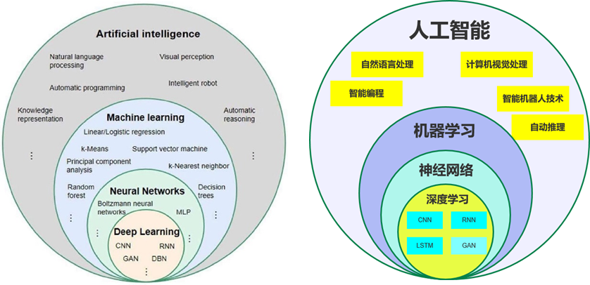
AI : Artificial Intelligence,旨在研究、开发能够模拟、延伸和扩展人类智能的理论、方法、技术及应用系统,是一种拥有自主学习和推理能力的技术。它模仿人类大脑某些功能,包括感知、学习、理解、决策和问题解决。
AI本质
-
本质是数学计算
-
数学是理论关键
-
计算机是实现关键:算力
-
新的有效算法,需要更大的算力
NLP(说话,听)、CV(眼睛)、自动驾驶、机器人(肢体动作)、大模型
2. 人工智能实现过程
三要素:数据、网络、算力
① 神经网络:找到合适的数学公式;
② 训练:用已有数据训练网络,目标是求最优解;
③ 推理:用模型预测新样本;
3. 术语关系图
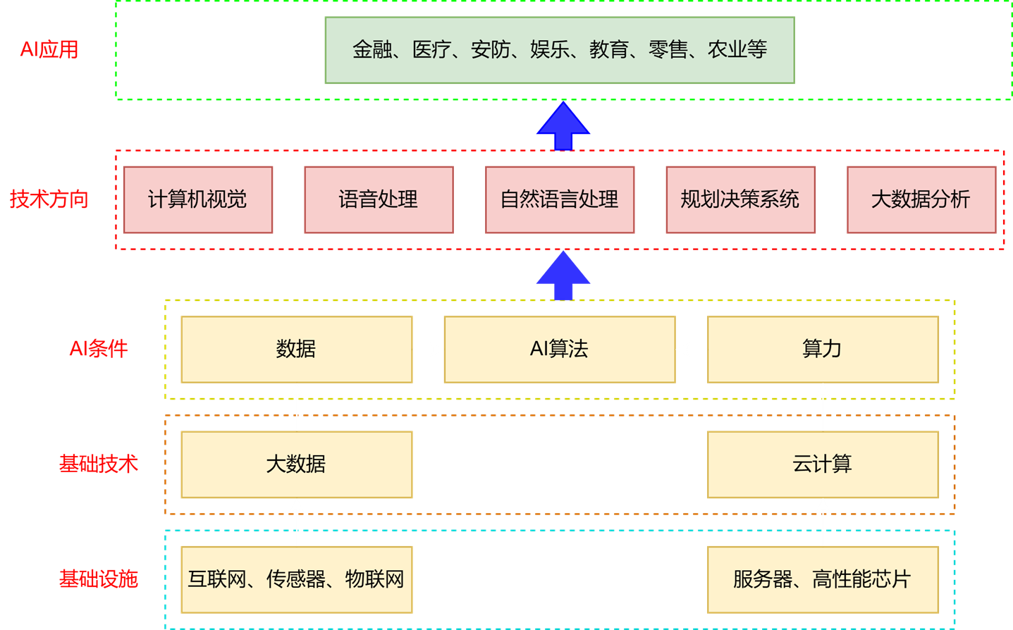
4. AI产业大生态
二、初识Torch
PyTorch,简称Torch,主流的经典的深度学习框架,如果你只想掌握一个深度学习框架,那就毫不犹豫的选择他吧!

翻译:用Torch进行深度学习。
通过本阶段的学习, 各位大佬将熟练掌握PyTorch的使用,为后续学习网络搭建、模型训练等打下基础。
1. 生涩的简介
PyTorch是一个基于Python的深度学习框架,它提供了一种灵活、高效、易于学习的方式来实现深度学习模型。PyTorch最初由Facebook开发,被广泛应用于计算机视觉、自然语言处理、语音识别等领域。
PyTorch使用张量(tensor)来表示数据,可以轻松地处理大规模数据集,且可以在GPU上加速。
PyTorch提供了许多高级功能,如自动微分(automatic differentiation)、自动求导(automatic gradients)等,这些功能可以帮助我们更好地理解模型的训练过程,并提高模型训练效率。
2. 多彩的江湖
除了PyTorch,还有很多其它常见的深度学习框架:
-
TensorFlow: Google开发,广泛应用于学术界和工业界。TensorFlow提供了灵活的构建、训练和部署功能,并支持分布式计算。
-
Keras: Keras是一个高级神经网络API,已整合到TensorFlow中。
-
PaddlePaddle: PaddlePaddle(飞桨)是百度推出的开源深度学习平台,旨在为开发者提供一个易用、高效的深度学习开发框架。
-
MXNet:由亚马逊开发,具有高效的分布式训练支持和灵活的混合编程模型。
-
Caffe:具有速度快、易用性高的特点,主要用于图像分类和卷积神经网络的相关任务。
-
CNTK :由微软开发的深度学习框架,提供了高效的训练和推理性能。CNTK支持多种语言的接口,包括Python、C++和C#等。
-
Chainer:由Preferred Networks开发的开源深度学习框架,采用动态计算图的方式。
三、Tensor概述
PyTorch会将数据封装成张量(Tensor)进行计算,所谓张量就是元素为相同类型的多维矩阵。
张量可以在 GPU 上加速运行。
1. 概念
张量是一个多维数组,通俗来说可以看作是扩展了标量、向量、矩阵的更高维度的数组。张量的维度决定了它的形状(Shape),例如:
-
标量 是 0 维张量,如
a = torch.tensor(5) -
向量 是 1 维张量,如
b = torch.tensor([1, 2, 3]) -
-
其中
[1,2,3]:有三个维度,即为0,1,2
-
-
矩阵 是 2 维张量,如
c = torch.tensor([[1, 2], [3, 4]]) -
更高维度的张量,如3维、4维等,通常用于表示图像、视频数据等复杂结构。
个人理解:张量就是数组,数组中的元素下标就是张量的维度
2. 特点
-
动态计算图:PyTorch 支持动态计算图,这意味着在每一次前向传播时,计算图是即时创建的。
-
GPU 支持:PyTorch 张量可以通过
.to('cuda')移动到 GPU 上进行加速计算。 -
自动微分:通过
autograd模块,PyTorch 可以自动计算张量运算的梯度,这对深度学习中的反向传播算法非常重要。
3. 数据类型
PyTorch中有3种数据类型:浮点数、整数、布尔。其中,浮点数和整数又分为8位、16位、32位、64位,加起来共9种。
为什么要分为8位、16位、32位、64位呢?
场景不同,对数据的精度和速度要求不同。通常,移动或嵌入式设备追求速度,对精度要求相对低一些。精度越高,往往效果也越好,自然硬件开销就比较高。
四、Tensor的创建
在Torch中张量以 "类" 的形式封装起来,对张量的一些运算、处理的方法被封装在类中,官方文档:
torch — PyTorch 2.8 documentation
1. 基本创建方式
以下讲的创建tensor的函数中有两个有默认值的参数dtype和device, 分别代表数据类型和计算设备,可以通过属性dtype和device获取。
1.1 torch.tensor
注意这里的tensor是小写,该API是根据指定的数据创建张量。
import torch
import numpy as np


def test001():
    # 1. 用标量创建张量
    tensor = torch.tensor(5)
    print(tensor.shape)

    # 2. 使用numpy随机一个数组创建张量
    tensor = torch.tensor(np.random.randn(3, 5))
    print(tensor)
    print(tensor.shape)

    # 3. 根据list创建tensor
    tensor = torch.tensor([[1, 2, 3], [4, 5, 6]])
    print(tensor)
    print(tensor.shape)
    print(tensor.dtype)


if __name__ == '__main__':
    test001()
注:如果出现如下错误:
UserWarning: Failed to initialize NumPy: _ARRAY_API not found一般是因为numpy和pytorch版本不兼容,可以降低numpy版本,步骤如下:
1.anaconda prompt中切换虚拟环境:
conda activate 虚拟环境名称2.卸载numpy:
pip uninstall numpy3.安装低版本的numpy:
pip install numpy==1.26.01.2 torch.Tensor
注意这里的Tensor是大写,该API根据形状创建张量,其也可用来创建指定数据的张量。
import torch
import numpy as np

def test002():
    # 1. 根据形状创建张量
    tensor1 = torch.Tensor(2, 3)
    print(tensor1)
    # 2. 也可以是具体的值
    tensor2 = torch.Tensor([[1, 2, 3], [4, 5, 6]])
    print(tensor2, tensor2.shape, tensor2.dtype)

    tensor3 = torch.Tensor([10])
    print(tensor3, tensor3.shape, tensor3.dtype)

    # 指定tensor数据类型
    tensor1 = torch.Tensor([1,2,3]).short()
    print(tensor1)

    tensor1 = torch.Tensor([1,2,3]).int()
    print(tensor1)

    tensor1 = torch.Tensor([1,2,3]).float()
    print(tensor1)

    tensor1 = torch.Tensor([1,2,3]).double()
    print(tensor1)


if __name__ == "__main__":
    test002()
torch.Tensor与torch.tensor区别
| 特性 | torch.Tensor() |
torch.tensor() |
|---|---|---|
| 数据类型推断 | 强制转为 torch.float32 |
根据输入数据自动推断(如整数→int64) |
显式指定 dtype |
不支持 | 支持(如 dtype=torch.float64) |
| 设备指定 | 不支持 | 支持(如 device='cuda') |
| 输入为张量时的行为 | 创建新副本(不继承原属性) | 默认共享数据(除非 copy=True) |
| 推荐使用场景 | 需要快速创建浮点张量 | 需要精确控制数据类型或设备 |
1.3 torch.IntTensor
用于创建指定类型的张量,还有诸如Torch.FloatTensor、 torch.DoubleTensor、 torch.LongTensor......等。
如果数据类型不匹配,那么在创建的过程中会进行类型转换,要尽可能避免,防止数据丢失。
import torch

def test003():
    # 1. 创建指定形状的张量
    tt1 = torch.IntTensor(2, 3)
    print(tt1)

    tt2 = torch.FloatTensor(3, 3)
    print(tt2, tt2.dtype)
    tt3 = torch.DoubleTensor(3, 3)
    print(tt3, tt3.dtype)
    tt4 = torch.LongTensor(3, 3)
    print(tt4, tt4.dtype)
    tt5 = torch.ShortTensor(3, 3)
    print(tt5, tt5.dtype)


if __name__ == "__main__":
    test003()
2. 创建线性和随机张量
在 PyTorch 中,可以轻松创建线性张量和随机张量。
2.1 创建线性张量
使用torch.arange 和 torch.linspace 创建线性张量:
import torch
import numpy as np

# 不用科学计数法打印
torch.set_printoptions(sci_mode=False)


def test004():
    # 1. 创建线性张量
    r1 = torch.arange(0, 10, 2)
    print(r1)
    # 2. 在指定空间按照元素个数生成张量:等差
    r2 = torch.linspace(3, 10, 10)
    print(r2)

    r2 = torch.linspace(3, 10000000, 10)
    print(r2)


if __name__ == "__main__":
    test004()
2.2 随机张量
使用torch.randn 创建随机张量。
2.2.1 随机数种子
随机数种子(Random Seed)是一个用于初始化随机数生成器的数值。随机数生成器是一种算法,用于生成一个看似随机的数列,但如果使用相同的种子进行初始化,生成器将产生相同的数列。
随机数种子的设置和获取:
import torch


def test001():
    # 设置随机数种子
    torch.manual_seed(123)

    # 获取随机数种子
    print(torch.initial_seed())


if __name__ == "__main__":
    test001()
2.2.2 随机张量
在 PyTorch 中,种子影响所有与随机性相关的操作,包括张量的随机初始化、数据的随机打乱、模型的参数初始化等。通过设置随机数种子,可以做到模型训练和实验结果在不同的运行中进行复现。
import torch


def test001():
    # 1. 设置随机数种子
    torch.manual_seed(123)

    # 2. 获取随机数种子,需要查看种子时调用
    print(torch.initial_seed())

    # 3. 生成随机张量,均匀分布(范围 [0, 1))
    # 创建2个样本,每个样本3个特征
    print(torch.rand(2, 3))

    # 4. 生成随机张量:标准正态分布(均值 0,标准差 1)
    print(torch.randn(2, 3))

    # 5. 原生服从正态分布:均值为2, 方差为3,形状为1*4的正态分布
    print(torch.normal(mean=2, std=3, size=(1, 4)))


if __name__ == "__main__":
    test001()
注:不设置随机种子时,每次打印的结果不一样。
五、Tensor常见属性
张量有device、dtype、shape等常见属性,知道这些属性对我们认识Tensor很有帮助。
1. 获取属性
掌握代码调试就是掌握了一切~
import torch


def test001():
    data = torch.tensor([1, 2, 3])
    print(data.dtype, data.device, data.shape)


if __name__ == "__main__":
    test001()
2. 切换设备
默认在cpu上运行,可以显式的切换到GPU:不同设备上的数据是不能相互运算的。
import torch


def test001():
    data = torch.tensor([1, 2, 3])
    print(data.dtype, data.device, data.shape)

    # 把数据切换到GPU进行运算
    device = "cuda" if torch.cuda.is_available() else "cpu"
    data = data.to(device)
    print(data.device)


if __name__ == "__main__":
    test001()
或者使用cuda进行切换:
data = data.cuda()当然也可以直接创建在GPU上:
# 直接在GPU上创建张量
data = torch.tensor([1, 2, 3], device='cuda')
print(data.device)
3. 类型转换
在训练模型或推理时,类型转换也是张量的基本操作,是需要掌握的。
import torch


def test001():
    data = torch.tensor([1, 2, 3])
    print(data.dtype)  # torch.int64

    # 1. 使用type进行类型转换
    data = data.type(torch.float32)
    print(data.dtype)  # float32
    data = data.type(torch.float16)
    print(data.dtype)  # float16

    # 2. 使用类型方法
    data = data.float()
    print(data.dtype)  # float32
    # 16 位浮点数,torch.float16,即半精度
    data = data.half()
    print(data.dtype)  # float16
    data = data.double()
    print(data.dtype)  # float64
    data = data.long()
    print(data.dtype)  # int64
    data = data.int()
    print(data.dtype)  # int32

    #  使用dtype属性
    data = torch.tensor([1, 2, 3], dtype=torch.half)
    print(data.dtype)


if __name__ == "__main__":
    test001()
六、Tensor数据转换
1. Tensor与Numpy
Tensor和Numpy都是常见数据格式,惹不起~
1.1 张量转Numpy
此时分内存共享和内存不共享~
1.1.1 浅拷贝
调用numpy()方法可以把Tensor转换为Numpy,此时内存是共享的。
import torch


def test003():
    # 1. 张量转numpy
    data_tensor = torch.tensor([[1, 2, 3], [4, 5, 6]])
    data_numpy = data_tensor.numpy()
    print(type(data_tensor), type(data_numpy))
    # 2. 他们内存是共享的
    data_numpy[0, 0] = 100
    print(data_tensor, data_numpy)


if __name__ == "__main__":
    test003()
1.1.2 深拷贝
使用copy()方法可以避免内存共享:
import torch


def test003():
    # 1. 张量转numpy
    data_tensor = torch.tensor([[1, 2, 3], [4, 5, 6]])

    # 2. 使用copy()避免内存共享
    data_numpy = data_tensor.numpy().copy()
    print(type(data_tensor), type(data_numpy))

    # 3. 此时他们内存是不共享的
    data_numpy[0, 0] = 100
    print(data_tensor, data_numpy)


if __name__ == "__main__":
    test003()
1.2 Numpy转张量
也可以分为内存共享和不共享~
1.2.1 浅拷贝
from_numpy方法转Tensor默认是内存共享的
import numpy as np
import torch


def test006():
    # 1. numpy转张量
    data_numpy = np.array([[1, 2, 3], [4, 5, 6]])
    data_tensor = torch.from_numpy(data_numpy)
    print(type(data_tensor), type(data_numpy))

    # 2. 他们内存是共享的
    data_tensor[0, 0] = 100
    print(data_tensor, data_numpy)


if __name__ == "__main__":
    test006()
1.2.2 深拷贝
使用传统的torch.tensor()则内存是不共享的~
import numpy as np
import torch


def test006():
    # 1. numpy转张量
    data_numpy = np.array([[1, 2, 3], [4, 5, 6]])
    data_tensor = torch.tensor(data_numpy)
    print(type(data_tensor), type(data_numpy))

    # 2. 内存是不共享的
    data_tensor[0, 0] = 100
    print(data_tensor, data_numpy)


if __name__ == "__main__":
    test006()
七、Tensor常见操作
在深度学习中,Tensor是一种多维数组,用于存储和操作数据,我们需要掌握张量各种运算。
1. 获取元素值
我们可以把单个元素tensor转换为Python数值,这是非常常用的操作
import torch


def test002():
    data = torch.tensor([18])
    print(data.item())
    pass


if __name__ == "__main__":
    test002()
注意:
-
和Tensor的维度没有关系,都可以取出来!
-
如果有多个元素则报错;
-
仅适用于CPU张量,如果张量在GPU上,需先移动到CPU
-
gpu_tensor = torch.tensor([1.0], device='cuda')
value = gpu_tensor.cpu().item()  # 先转CPU再提取
2. 元素值运算
常见的加减乘除次方取反开方等各种操作,带有_的方法则会替换原始值。
import torch


def test001():
    # 生成范围 [0, 10) 的 2x3 随机整数张量
    data = torch.randint(0, 10, (2, 3))
    print(data)

    # 元素级别的加减乘除:不修改原始值,返回新对象
    print(data.add(1))
    print(data.sub(1))
    print(data.mul(2))
    print(data.div(3))
    print(data.pow(2))

    # 元素级别的加减乘除:修改原始值
    data = data.float()
    data.add_(1)
    data.sub_(1)
    data.mul_(2)
    data.div_(3.0)
    data.pow_(2)
    print(data)


if __name__ == "__main__":
    test001()
3. 阿达玛积
阿达玛积是指两个形状相同的矩阵或张量对应位置的元素相乘。它与矩阵乘法不同,矩阵乘法是线性代数中的标准乘法,而阿达玛积是逐元素操作。假设有两个形状相同的矩阵 A和 B,它们的阿达玛积 C=A∘B定义为:
其中:
-
Cij 是结果矩阵 C的第 i行第 j列的元素。
-
Aij和 Bij分别是矩阵 A和 B的第 i行第 j 列的元素。
在 PyTorch 中,可以使用mul函数或者*来实现;
import torch


def test001():
    data1 = torch.tensor([[1, 2, 3], [4, 5, 6]])
    data2 = torch.tensor([[2, 3, 4], [2, 2, 3]])
    print(data1 * data2)


def test002():
    data1 = torch.tensor([[1, 2, 3], [4, 5, 6]])
    data2 = torch.tensor([[2, 3, 4], [2, 2, 3]])
    print(data1.mul(data2))


if __name__ == "__main__":
    test001()
    test002()
4. Tensor相乘
矩阵乘法是线性代数中的一种基本运算,用于将两个矩阵相乘,生成一个新的矩阵。
假设有两个矩阵:
-
矩阵 A的形状为 m×n(m行 n列)。
-
矩阵 B的形状为 n×p(n行 p列)。
矩阵 A和 B的乘积 C=A×B是一个形状为 m×p的矩阵,其中 C的每个元素 Cij,计算 A的第 i行与 B的第 j列的点积。计算公式为:
矩阵乘法运算要求如果第一个矩阵的shape是 (N, M),那么第二个矩阵 shape必须是 (M, P),最后两个矩阵点积运算的shape为 (N, P)。
在 PyTorch 中,使用@或者matmul完成Tensor的乘法。
import torch


def test006():
    data1 = torch.tensor([
        [1, 2, 3],
        [4, 5, 6]
    ])
    data2 = torch.tensor([
        [3, 2],
        [2, 3],
        [5, 3]
    ])
    print(data1 @ data2)
    print(data1.matmul(data2))


if __name__ == "__main__":
    test006()
5. 形状操作
在 PyTorch 中,张量的形状操作是非常重要的,因为它允许你灵活地调整张量的维度和结构,以适应不同的计算需求。
5.1 reshape
可以用于将张量转换为不同的形状,但要确保转换后的形状与原始形状具有相同的元素数量。
import torch


def test001():
    data = torch.randint(0, 10, (4, 3))
    print(data)
    # 1. 使用reshape改变形状
    data = data.reshape(2, 2, 3)
    print(data)

    # 2. 使用-1表示自动计算
    data = data.reshape(2, -1)
    print(data)


if __name__ == "__main__":
    test001()
5.2 view
view进行形状变换的特征:
-
张量在内存中是连续的(前提条件);
-
返回的是
原始张量视图,不重新分配内存,效率更高; -
如果张量在内存中不连续,view 将无法执行,并抛出错误。
5.2.1 内存连续性
张量的内存布局决定了其元素在内存中的存储顺序。对于多维张量,内存布局通常按照最后一个维度优先的顺序存储,即先存列,后存行。例如,对于一个二维张量 A,其形状为 (m, n),其内存布局是先存储第 0 行的所有列元素,然后是第 1 行的所有列元素,依此类推。
如果张量的内存布局与形状完全匹配,并且没有被某些操作(如转置、索引等)打乱,那么这个张量就是连续的。
PyTorch 的大多数操作都是基于 C 顺序的,我们在进行变形或转置操作时,很容易造成内存的不连续性。
import torch


def test001():
    tensor = torch.tensor([[1, 2, 3], [4, 5, 6]])
    print("正常情况下的张量:", tensor.is_contiguous())

    # 对张量进行转置操作
    tensor = tensor.t()
    print("转置操作的张量:", tensor.is_contiguous())
    print(tensor)
    # 此时使用view进行变形操作
    tensor = tensor.view(2, -1)
    print(tensor)


if __name__ == "__main__":
    test001()
执行结果:
正常情况下的张量: True
转置操作的张量: False
tensor([[1, 4],
        [2, 5],
        [3, 6]])
Traceback (most recent call last):
  File "e:\01.深度学习\01.参考代码\14.PyTorch.内存连续性.py", line 20, in <module>
    test001()
  File "e:\01.深度学习\01.参考代码\14.PyTorch.内存连续性.py", line 13, in test001
    tensor = tensor.view(2, -1)
RuntimeError: view size is not compatible with input tensor's size and stride (at least one dimension spans across two contiguous subspaces). Use .reshape(...) instead.
5.2.2 和reshape比较
view:高效,但需要张量在内存中是连续的;
reshape:更灵活,但涉及内存复制;
5.2.3 view变形操作
import torch


def test002():
    tensor = torch.tensor([[1, 2, 3], [4, 5, 6]])
    # 将 2x3 的张量转换为 3x2
    reshaped_tensor = tensor.view(3, 2)
    print(reshaped_tensor)

    # 自动推断一个维度
    reshaped_tensor = tensor.view(-1, 2)
    print(reshaped_tensor)


if __name__ == "__main__":
    test002()
5.3 transpose
transpose 用于交换张量的两个维度,注意,是2个维度,它返回的是原张量的视图(dim:维度)。
torch.transpose(input, dim0, dim1)参数
-
input: 输入的张量。
-
dim0: 要交换的第一个维度。
-
dim1: 要交换的第二个维度。
import torch


def test003():
    data = torch.randint(0, 10, (3, 4, 5))
    print(data, data.shape)
    # 使用transpose进行形状变换
    transpose_data = torch.transpose(data,0,1)
    # transpose_data = data.transpose(0, 1)
    print(transpose_data, transpose_data.shape)


if __name__ == "__main__":
    test003()
ranspose 返回新张量,原张量不变
转置后的张量可能是非连续的(is_contiguous() 返回 False),如果需要连续内存(如某些操作要求),可调用 .contiguous():
y = x.transpose(0, 1).contiguous()5.4 permute
它通过重新排列张量的维度来返回一个新的张量,不改变张量的数据,只改变维度的顺序。
torch.permute(input, dims)参数
-
input: 输入的张量。
-
dims: 一个整数元组,表示新的维度顺序。
import torch


def test004():
    data = torch.randint(0, 10, (3, 4, 5))
    print(data, data.shape)
    # 使用permute进行多维度形状变换
    permute_data = data.permute(1, 2, 0)
    print(permute_data, permute_data.shape)


if __name__ == "__main__":
    test004()
和 transpose 一样,permute 返回新张量,原张量不变。
重排后的张量可能是非连续的(is_contiguous() 返回 False),必要时需调用 .contiguous():
y = x.permute(2, 1, 0).contiguous()维度顺序必须合法:dims 中的维度顺序必须包含所有原始维度,且不能重复或遗漏。例如,对于一个形状为 (2, 3, 4) 的张量,dims=(2, 0, 1) 是合法的,但 dims=(0, 1) 或 dims=(0, 1, 2, 3) 是非法的。
与 transpose() 的对比
| 特性 | permute() | transpose() |
|---|---|---|
| 功能 | 可以同时调整多个维度的顺序 | 只能交换两个维度的顺序 |
| 灵活性 | 更灵活 | 较简单 |
| 使用场景 | 适用于多维张量 | 适用于简单的维度交换 |
5.5 升维和降维
在后续的网络学习中,升维和降维是常用操作,需要掌握。
-
unsqueeze:用于在指定位置插入一个大小为 1 的新维度。
-
squeeze:用于移除所有大小为 1 的维度,或者移除指定维度的大小为 1 的维度。
5.5.1 squeeze降维
torch.squeeze(input, dim=None)参数
-
input: 输入的张量。
-
dim (可选): 指定要移除的维度。如果指定了 dim,则只移除该维度(前提是该维度大小为 1);如果不指定,则移除所有大小为 1 的维度。
import torch


def test006():
    data = torch.randint(0, 10, (1, 4, 5, 1))
    print(data, data.shape)

    # 进行降维操作
    data1 = data.squeeze(0).squeeze(-1)
    print(data.shape)

    # 移除所有大小为 1 的维度
	data2 = torch.squeeze(data)

    # 尝试移除第 1 维(大小为 3,不为 1,不会报错,张量保持不变。)
	data3 = torch.squeeze(data, dim=1)
	print("尝试移除第 1 维后的形状:", data3.shape)


if __name__ == "__main__":
    test006()
5.5.2 unsqueeze升维
torch.unsqueeze(input, dim)参数
-
input: 输入的张量。
-
dim: 指定要增加维度的位置(从 0 开始索引)
import torch


def test007():
    data = torch.randint(0, 10, (32, 32, 3))
    print(data.shape)
    # 升维操作
    data = data.unsqueeze(0)
    print(data.shape)


if __name__ == "__main__":
    test007()
6. 广播机制
广播机制允许在对不同形状的张量进行计算,而无需显式地调整它们的形状。广播机制通过自动扩展较小维度的张量,使其与较大维度的张量兼容,从而实现按元素计算。
6.1 广播机制规则
广播机制需要遵循以下规则:
-
每个张量的维度至少为1
-
满足右对齐
6.2 广播案例
1D和2D张量广播
import torch


def test006():
    data1d = torch.tensor([1, 2, 3])
    data2d = torch.tensor([[4], [2], [3]])
    print(data1d.shape, data2d.shape)
    # 进行计算:会自动进行广播机制
    print(data1d + data2d)


if __name__ == "__main__":
    test006()
输出:
torch.Size([3]) torch.Size([3, 1])
    tensor([[5, 6, 7],
            [3, 4, 5],
            [4, 5, 6]])
2D 和 3D 张量广播
广播机制会根据需要对两个张量进行形状扩展,以确保它们的形状对齐,从而能够进行逐元素运算。广播是双向奔赴的。
import torch


def test001():
    # 2D 张量
    a = torch.tensor([[1, 2, 3], [4, 5, 6]])

    # 3D 张量
    b = torch.tensor([[[2, 3, 4]], [[5, 6, 7]]])
    print(a.shape, b.shape)

    # 进行运算
    result = a + b
    print(result, result.shape)


if __name__ == "__main__":
    test001()
执行结果:
torch.Size([2, 3]) torch.Size([2, 1, 3])
tensor([[[ 3,  5,  7],
         [ 6,  8, 10]],

        [[ 6,  8, 10],
         [ 9, 11, 13]]]) torch.Size([2, 2, 3])
最终参与运算的a和b形式如下:
# 2D 张量
a = torch.tensor([[[1, 2, 3], [4, 5, 6]],[[1, 2, 3], [4, 5, 6]]])

# 3D 张量
b = torch.tensor([[[2, 3, 4], [2, 3, 4]], [[5, 6, 7], [5, 6, 7]]])
八、自动微分
自动微分模块torch.autograd负责自动计算张量操作的梯度,具有自动求导功能。自动微分模块是构成神经网络训练的必要模块,可以实现网络权重参数的更新,使得反向传播算法的实现变得简单而高效。
1. 基础概念
-
张量
Torch中一切皆为张量,属性requires_grad决定是否对其进行梯度计算。默认是 False,如需计算梯度则设置为True。
-
计算图:
torch.autograd通过创建一个动态计算图来跟踪张量的操作,每个张量是计算图中的一个节点,节点之间的操作构成图的边。
在 PyTorch 中,当张量的 requires_grad=True 时,PyTorch 会自动跟踪与该张量相关的所有操作,并构建计算图。每个操作都会生成一个新的张量,并记录其依赖关系。当设置为
True时,表示该张量在计算图中需要参与梯度计算,即在反向传播(Backpropagation)过程中会自动计算其梯度;当设置为False时,不会计算梯度。例如:
在上述代码中,x 和 y 是输入张量,即叶子节点,z 是中间结果,loss 是最终输出。每一步操作都会记录依赖关系:
z = x * y:z 依赖于 x 和 y。
loss = z.sum():loss 依赖于 z。
这些依赖关系形成了一个动态计算图,如下所示:
      x       y
       \     /
        \   /
         \ /
          z
          |
          |
          v
loss叶子节点:
在 PyTorch 的自动微分机制中,叶子节点(leaf node) 是计算图中:
-
由用户直接创建的张量,并且它的 requires_grad=True。
-
这些张量是计算图的起始点,通常作为模型参数或输入变量。
特征:
-
没有由其他张量通过操作生成。
-
如果参与了计算,其梯度会存储在 leaf_tensor.grad 中。
-
默认情况下,叶子节点的梯度不会自动清零,需要显式调用 optimizer.zero_grad() 或 x.grad.zero_() 清除。
如何判断一个张量是否是叶子节点?
通过 tensor.is_leaf 属性,可以判断一个张量是否是叶子节点。
x = torch.tensor([1.0, 2.0, 3.0], requires_grad=True)  # 叶子节点
y = x ** 2  # 非叶子节点(通过计算生成)
z = y.sum()

print(x.is_leaf)  # True
print(y.is_leaf)  # False
print(z.is_leaf)  # False
叶子节点与非叶子节点的区别
| 特性 | 叶子节点 | 非叶子节点 |
|---|---|---|
| 创建方式 | 用户直接创建的张量 | 通过其他张量的运算生成 |
| is_leaf 属性 | True | False |
| 梯度存储 | 梯度存储在 .grad 属性中,会参与计算 | 梯度不会存储在 .grad,只能通过反向传播传递,不会参与计算 |
| 是否参与计算图 | 是计算图的起点 | 是计算图的中间或终点 |
| 删除条件 | 默认不会被删除 | 在反向传播后,默认被释放(除非 retain_graph=True) |
detach():张量 x 从计算图中分离出来,返回一个新的张量,与 x 共享数据,但不包含计算图(即不会追踪梯度)。
特点:
-
返回的张量是一个新的张量,与原始张量共享数据。
-
对 x.detach() 的操作不会影响原始张量的梯度计算。
-
推荐使用 detach(),因为它更安全,且在未来版本的 PyTorch 中可能会取代 data。
x = torch.tensor([1.0, 2.0, 3.0], requires_grad=True)
y = x.detach()  # y 是一个新张量,不追踪梯度

y += 1  # 修改 y 不会影响 x 的梯度计算
print(x)  # tensor([1., 2., 3.], requires_grad=True)
print(y) # tensor([2., 3., 4.])-
反向传播
使用tensor.backward()方法执行反向传播,从而计算张量的梯度。这个过程会自动计算每个张量对损失函数的梯度。例如:调用 loss.backward() 从输出节点 loss 开始,沿着计算图反向传播,计算每个节点的梯度。
-
梯度
计算得到的梯度通过tensor.grad访问,这些梯度用于优化模型参数,以最小化损失函数。
2. 计算梯度
使用tensor.backward()方法执行反向传播,从而计算张量的梯度
2.1 标量梯度计算
参考代码如下:
import torch


def test001():
    # 1. 创建张量:必须为浮点类型
    x = torch.tensor(1.0, requires_grad=True)


    # 2. 操作张量
    y = x ** 2

    # 3. 计算梯度,也就是反向传播
    y.backward()

    # 4. 读取梯度值
    print(x.grad)  # 输出: tensor(2.)


if __name__ == "__main__":
    test001()
2.2 向量梯度计算
案例:
def test003():
    # 1. 创建张量:必须为浮点类型
    x = torch.tensor([1.0, 2.0, 3.0], requires_grad=True)

    # 2. 操作张量
    y = x ** 2

    # 3. 计算梯度,也就是反向传播
    y.backward()

    # 4. 读取梯度值
    print(x.grad)


if __name__ == "__main__":
    test003()
错误预警:RuntimeError: grad can be implicitly created only for scalar outputs
由于 y 是一个向量,我们需要提供一个与 y 形状相同的向量作为 backward() 的参数,这个参数通常被称为 梯度张量(gradient tensor),它表示 y 中每个元素的梯度。
def test003():
    # 1. 创建张量:必须为浮点类型
    x = torch.tensor([1.0, 2.0, 3.0], requires_grad=True)

    # 2. 操作张量
    y = x ** 2

    # 3. 计算梯度,也就是反向传播
    y.backward(torch.tensor([1.0, 1.0, 1.0]))

    # 4. 读取梯度值
    print(x.grad)

    # 输出
    # tensor([2., 4., 6.])


if __name__ == "__main__":
    test003()
我们也可以将向量 y 通过一个标量损失函数(如 y.mean())转换为一个标量,反向传播时就不需要提供额外的梯度向量参数了。这是因为标量的梯度是明确的,直接调用 .backward() 即可。
import torch


def test002():
    # 1. 创建张量:必须为浮点类型
    x = torch.tensor([1.0, 2.0, 3.0], requires_grad=True)

    # 2. 操作张量
    y = x ** 2

    # 3. 损失函数
    loss = y.mean()

    # 4. 计算梯度,也就是反向传播
    loss.backward()

    # 5. 读取梯度值
    print(x.grad)


if __name__ == "__main__":
    test002()
调用 loss.backward() 从输出节点 loss 开始,沿着计算图反向传播,计算每个节点的梯度。
损失函数,其中 n=3。
对于每个 ,其梯度为
对于每个 ,其梯度为
所以,x.grad 的值为:
2.3 多标量梯度计算
参考代码如下
import torch


def test003():
    # 1. 创建两个标量
    x1 = torch.tensor(5.0, requires_grad=True, dtype=torch.float64)
    x2 = torch.tensor(3.0, requires_grad=True, dtype=torch.float64)

    # 2. 构建运算公式
    y = x1 ** 2 + 2 * x2 + 7

    # 3. 计算梯度,也就是反向传播
    y.backward()

    # 4. 读取梯度值
    print(x1.grad, x2.grad)

    # 输出:
    # tensor(10., dtype=torch.float64) tensor(2., dtype=torch.float64)


if __name__ == "__main__":
    test003()
2.4 多向量梯度计算
代码参考如下
import torch


def test004():
    # 创建两个张量,并设置 requires_grad=True
    x = torch.tensor([1.0, 2.0, 3.0], requires_grad=True)
    y = torch.tensor([4.0, 5.0, 6.0], requires_grad=True)

    # 前向传播:计算 z = x * y
    z = x * y

    # 前向传播:计算 loss = z.sum()
    loss = z.sum()

    # 查看前向传播的结果
    print("z:", z)  # 输出: tensor([ 4., 10., 18.], grad_fn=<MulBackward0>)
    print("loss:", loss)  # 输出: tensor(32., grad_fn=<SumBackward0>)

    # 反向传播:计算梯度
    loss.backward()

    # 查看梯度
    print("x.grad:", x.grad)  # 输出: tensor([4., 5., 6.])
    print("y.grad:", y.grad)  # 输出: tensor([1., 2., 3.])


if __name__ == "__main__":
    test004()
3. 梯度上下文控制
梯度计算的上下文控制和设置对于管理计算图、内存消耗、以及计算效率至关重要。下面我们学习下Torch中与梯度计算相关的一些主要设置方式。
3.1 控制梯度计算
梯度计算是有性能开销的,有些时候我们只是简单的运算,并不需要梯度
import torch


def test001():
    x = torch.tensor(10.5, requires_grad=True)
    print(x.requires_grad)  # True

    # 1. 默认y的requires_grad=True
    y = x**2 + 2 * x + 3
    print(y.requires_grad)  # True

    # 2. 如果不需要y计算梯度-with进行上下文管理
    with torch.no_grad():
        y = x**2 + 2 * x + 3
    print(y.requires_grad)  # False

    # 3. 如果不需要y计算梯度-使用装饰器
    @torch.no_grad()
    def y_fn(x):
        return x**2 + 2 * x + 3

    y = y_fn(x)
    print(y.requires_grad)  # False

    # 4. 如果不需要y计算梯度-全局设置,需要谨慎
    torch.set_grad_enabled(False)
    y = x**2 + 2 * x + 3
    print(y.requires_grad)  # False


if __name__ == "__main__":
    test001()
3.2 累计梯度
默认情况下,当我们重复对一个自变量进行梯度计算时,梯度是累加的
import torch


def test002():
    # 1. 创建张量:必须为浮点类型
    x = torch.tensor([1.0, 2.0, 5.3], requires_grad=True)

    # 2. 累计梯度:每次计算都会累计梯度
    for i in range(3):
        y = x**2 + 2 * x + 7
        z = y.mean()
        z.backward()
        print(x.grad)


if __name__ == "__main__":
    test002()
输出结果:
tensor([1.3333, 2.0000, 4.2000])
思考:如果把 y = x**2 + 2 * x + 7放在循环外,会是什么结果?
会报错:
RuntimeError: Trying to backward through the graph a second time (or directly access saved tensors after they have already been freed). Saved intermediate values of the graph are freed when you call .backward() or autograd.grad(). Specify retain_graph=True if you need to backward through the graph a second time or if you need to access saved tensors after calling backward.PyTorch 的自动求导机制在调用 backward() 时,会计算梯度并将中间结果存储在计算图中。默认情况下,这些中间结果在第一次调用 backward() 后会被释放,以节省内存。如果再次调用 backward(),由于中间结果已经被释放,就会抛出这个错误。
3.3 梯度清零
大多数情况下是不需要梯度累加的,奇葩的事情还是需要解决的~
import torch


def test002():
    # 1. 创建张量:必须为浮点类型
    x = torch.tensor([1.0, 2.0, 5.3], requires_grad=True)

    # 2. 累计梯度:每次计算都会累计梯度
    for i in range(3):
        y = x**2 + 2 * x + 7
        z = y.mean()
        # 2.1 反向传播之前先对梯度进行清零
        if x.grad is not None:
            x.grad.zero_()

        z.backward()
        print(x.grad)


if __name__ == "__main__":
    test002()

# 输出:
# tensor([1.3333, 2.0000, 4.2000])
# tensor([1.3333, 2.0000, 4.2000])
# tensor([1.3333, 2.0000, 4.2000])
3.4 案例1-求函数最小值
通过梯度下降找到函数最小值
import torch
from matplotlib import pyplot as plt
import numpy as np


def test01():
    x = np.linspace(-10, 10, 100)
    y = x ** 2

    plt.plot(x, y)

    plt.show()


def test02():
    # 初始化自变量X
    x = torch.tensor([3.0], requires_grad=True, dtype=torch.float)
    # 迭代轮次
    epochs = 50
    # 学习率
    lr = 0.1

    list = []
    for i in range(epochs):
        # 计算函数表达式
        y = x ** 2

        # 梯度清零
        if x.grad is not None:
            x.grad.zero_()
        # 反向传播
        y.backward()
        # 梯度下降,不需要计算梯度,为什么?PyTorch通过自动微分(Autograd)机制自动完成了这一过程
        with torch.no_grad():
            #x = x - lr * x.grad,此处会返回一个新变量,则会失去原来的x的属性,比如requires_grad=True,所以会报错,因此需要做原地修改操作
            # 原地修改,修改的是原变量
            x -= lr * x.grad

        print('epoch:', i, 'x:', x.item(), 'y:', y.item())
        list.append((x.item(), y.item()))

    # 散点图,观察收敛效果
    x_list = [l[0] for l in list]
    y_list = [l[1] for l in list]

    plt.scatter(x=x_list, y=y_list)
    plt.show()


if __name__ == "__main__":
    test01()
    test02()
代码解释:
# 梯度下降,不需要计算梯度
with torch.no_grad():
    x -= lr * x.grad
如果去掉梯度控制会有什么结果?
代码中去掉梯度控制会报异常:
RuntimeError: a leaf Variable that requires grad is being used in an in-place operation.因为代码中x是叶子节点(叶子张量),是计算图的开始节点,并且设置需要梯度。在pytorch中不允许对需要梯度的叶子变量进行原地操作。因为这会破坏计算图,导致梯度计算错误。
在代码中,x 是一个叶子变量(即直接定义的张量,而不是通过其他操作生成的张量),并且设置了 requires_grad=True,因此不能直接通过 -= 进行原地更新。
解决方法
为了避免这个错误,可以使用以下两种方法:
方法 1:使用 torch.no_grad() 上下文管理器
在更新参数时,使用 torch.no_grad() 禁用梯度计算,然后通过非原地操作更新参数。
with torch.no_grad():
    a -= lr * a.grad
方法 2:使用 data 属性或detach()
通过 x.data 访问张量的数据部分(不涉及梯度计算),然后进行原地操作。
x.data -= lr * x.gradx.data返回一个与 a 共享数据的张量,但不包含计算图
特点:
-
返回的张量与原始张量共享数据。
-
对 x.data 的操作是原地操作(in-place),可能会影响原始张量的梯度计算。
-
不推荐使用 data,因为它可能会导致意外的行为(如梯度计算错误)。
能不能将代码修改为:
x = x - lr * x.grad答案是不能,以上代码中=左边的x变量是由右边代码计算得出的,就不是叶子节点了,从计算图中被剥离出来后没有了梯度,报错:
RuntimeError: element 0 of tensors does not require grad and does not have a grad_fn总结:以上方均不推荐,正确且推荐的做法是使用优化器,优化器后续会讲解。
3.5 案例2-函数参数求解-作业
import torch

def test02():
    # 定义数据
    x = torch.tensor([1, 2, 3, 4, 5], dtype=torch.float)
    y = torch.tensor([3, 5, 7, 9, 11], dtype=torch.float)

    # 定义模型参数 a 和 b,并初始化
    a = torch.tensor([1], dtype=torch.float, requires_grad=True)
    b = torch.tensor([1], dtype=torch.float, requires_grad=True)
    # 学习率
    lr = 0.1
    # 迭代轮次
    epochs = 100

    for epoch in range(epochs):


        # 前向传播:计算预测值 y_pred
        y_pred = a * x + b

        # 定义损失函数
        loss = ((y_pred - y) ** 2).mean()

        if a.grad is not None and b.grad is not None:
            a.grad.zero_()
            b.grad.zero_()

        # 反向传播:计算梯度
        loss.backward()

        # 梯度下降
        with torch.no_grad():
            a -= lr * a.grad
            b -= lr * b.grad

        if (epoch + 1) % 10 == 0:
            print(f'Epoch [{epoch + 1}/{epochs}], Loss: {loss.item():.4f}')

    print(f'a: {a.item()}, b: {b.item()}')


if __name__ == '__main__':
    test02()
代码逻辑:
在 PyTorch 中,所有的张量操作都会被记录在一个计算图中。对于代码:
y_pred = a * x + b
loss = ((y_pred - y) ** 2).mean()
计算图如下:
a → y_pred → loss
x ↗
b ↗-
a 和 b 是需要计算梯度的叶子张量(requires_grad=True)。
-
y_pred 是中间结果,依赖于 a 和 b。
-
loss 是最终的标量输出,依赖于 y_pred。
当调用 loss.backward() 时,PyTorch 会从 loss 开始,沿着计算图反向传播,计算 loss 对每个需要梯度的张量(如 a 和 b)的梯度。
1、计算 loss 对 y_pred 的梯度:
求损失函数关于 y_pred 的梯度(即偏导数组成的向量)。由于 loss 是 y_pred 的函数,我们需要对每个求偏导数,并将它们组合成一个向量。
应用链式法则和常数求导规则,对于每个 项,梯度向量的每个分量是:
将结果组合成一个向量,我们得到:
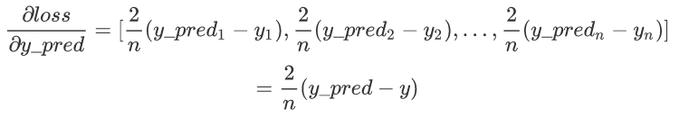
其中n=5,y_pred和y均为向量。
2、计算 y_pred 对 a 和 b 的梯度:
y_pred = a * x + b对 a 求导: ,x为向量
对 b 求导:
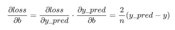
3、根据链式法则,loss 对 a 的梯度为:
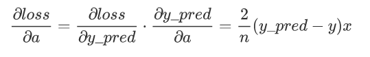
loss 对 b 的梯度为:
代码运行结果:
Epoch [10/100], Loss: 3020.7896
Epoch [20/100], Loss: 1550043.3750
Epoch [30/100], Loss: 795369408.0000
Epoch [40/100], Loss: 408125767680.0000
Epoch [50/100], Loss: 209420457869312.0000
Epoch [60/100], Loss: 107459239932329984.0000
Epoch [70/100], Loss: 55140217861896667136.0000
Epoch [80/100], Loss: 28293929961149737992192.0000
Epoch [90/100], Loss: 14518387713533614273593344.0000
Epoch [100/100], Loss: 7449779870375595263567855616.0000
a: -33038608105472.0, b: -9151163924480.0
损失函数在训练过程中越来越大,表明模型的学习过程出现了问题。这是因为学习率(Learning Rate)过大,参数更新可能会“跳过”最优值,导致损失函数在最小值附近震荡甚至发散。
解决方法:调小学习率,将lr=0.01
代码运行结果:
Epoch [10/100], Loss: 0.0965
Epoch [20/100], Loss: 0.0110
Epoch [30/100], Loss: 0.0099
Epoch [40/100], Loss: 0.0092
Epoch [50/100], Loss: 0.0086
Epoch [60/100], Loss: 0.0081
Epoch [70/100], Loss: 0.0075
Epoch [80/100], Loss: 0.0071
Epoch [90/100], Loss: 0.0066
Epoch [100/100], Loss: 0.0062
a: 1.9492162466049194, b: 1.1833451986312866
可以看出loss损失函数值在收敛,a接近2,b接近1
将epochs=500
代码运行结果:
Epoch [440/500], Loss: 0.0006
Epoch [450/500], Loss: 0.0006
Epoch [460/500], Loss: 0.0005
Epoch [470/500], Loss: 0.0005
Epoch [480/500], Loss: 0.0005
Epoch [490/500], Loss: 0.0004
Epoch [500/500], Loss: 0.0004
a: 1.986896276473999, b: 1.0473089218139648
a已经无限接近2,b无限接近1

欢迎加入北京社区
更多推荐


 35
35 0
0- 0


 已为社区贡献1条内容

所有评论(0)