下面给大家讲解AI生成式模型的主流解决方案，通过一个机器人写诗词的案例，带大家掌握GRU模型, char-to-char策略, GPT2, T5等技术使用。

第一部分：人工智能概述【主要分支】

通讯、感知与行动是现代人工智能的三个关键能力

• 计算机视觉(CV)
• 自然语言处理(NLP)
• 语音识别

语音识别

语音识别：指识别语音(说出的语言)并将其转换成对应文本的技术。相反的任务(文本转语音/TTS)也是这一领域内一个类似的研究主题。

当前阶段：进展颇丰，已经处于应用阶段很长时间

面临难题：声纹识别和 「鸡尾酒会效应」等一些特殊情况的难题。

自然语言处理

自然语言处理是指用计算机对自然语言的信息在单词级别，语义级别，篇章级别等进行处理。

最早的NLP任务 VS 最终的NLP任务

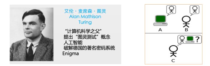
测试者与被测试者（一个人和一台机器）隔开的情况下，通过一些装置（如键盘）向被测试者随意提问。

测试准则（经过一段时间的聊天，比如15-30分钟），如果测试者不能确定被测试者是人还是机器，那么这台机器就通过了测试，并被认为具有人类智能。

深度学习定义

深度学习，利用人脑仿生的方式，一层一层的神经元，去自动模拟事物特征，进行预测对图片、声音的研究，大部分是使用深度学习技术。

NLP的几大基本任务

序列标注任务：

--- 分词

--- 词性标注

--- 命名实体识别

分类任务 ：

--- 文本类型的分类

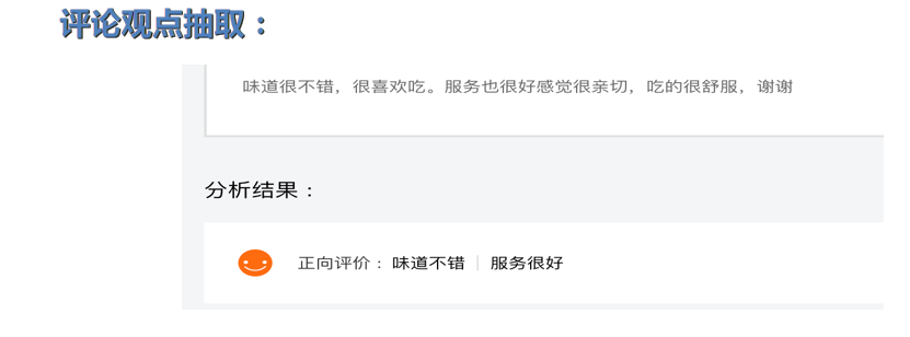
--- 情感分析

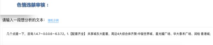
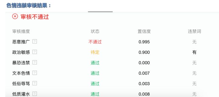
--- 舆情监控

句子关系任务：

--- 问答系统

--- 对话系统 (聊天机器人)

生成式任务 ：

--- 机器翻译

--- 文章摘要

第二部分：看图说话任务 (背景分析)

首先对比一下传统的机器翻译任务架构图(seq2seq)

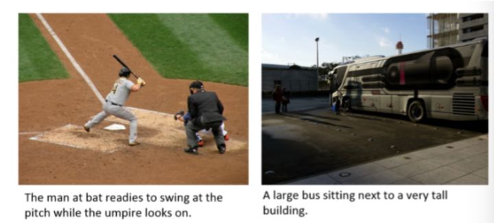
任务: 利用模型生成一段针对图片的描述文本, 这段文本和图片直接相关, 并抽取核心的语义, 比如下图所示。

如何找到和机器翻译任务的共同点？

数据预处理

训练数据集: MS-COCO

数据下载地址: Common Objects in Context

整个数据集分成两个部分:

1: 标注文件: annotations/captions_train2014.json

2: 图片文件: train2014/xxxx.jpg

# 使用InceptionV3预训练模型处理图片训练集数据
def load_image(image_path):
      # 以原生图片路径image_path为参数, 返回处理后的图片和图片路径
      # 读取原生图片路径 
      img = tf.io.read_file(image_path)
      # 对图片进行图片格式的解码, 颜色通道为3
      img = tf.image.decode_jpeg(img, channels=3)
      # 统一图片尺寸为299x299
      img = tf.image.resize(img, (299, 299))
      # 调用keras.applications.inception_v3中的preprocess_input方法对统一尺寸后的图片进行处理
      img = tf.keras.applications.inception_v3.preprocess_input(img)
      # 返回处理后的图片和对应的图片地址
      return img, image_path

经过刚才的函数预处理后的返回图片, 就是这个样子

top_k = 5000
# 使用tf.keras.preprocessing.text.Tokenizer方法实例化数值映射器
tokenizer = tf.keras.preprocessing.text.Tokenizer(num_words=top_k,
                                                  oov_token="<unk>",
                                                  filters='!"#$%&()*+.,-/:;=?@[\]^_`{|}~ ')

# 使用数值映射器拟合train_captions(用于训练的描述文本)
tokenizer.fit_on_texts(train_captions)
tokenizer.word_index['<pad>'] = 0
tokenizer.index_word[0] = '<pad>'

# 最后作用于描述文本得到对应的数值映射结果
train_seqs = tokenizer.texts_to_sequences(train_captions)
print("train_seqs:", train_seqs)

经过上面代码对文本描述进行预处理后, 所有的文本已经完成了数字化映射:

模型构建与训练

# 第一步是编码器, 基于seq2seq架构, 我们选择CNN为主体的编码器, 负责提取图片特征:

class CNN_Encoder(tf.keras.Model):
    def __init__(self, embedding_dim):
        super(CNN_Encoder, self).__init__()
        # 实例化一个全连接层
        self.fc = tf.keras.layers.Dense(embedding_dim)
    def call(self, x):
        # 使用全连接层
        x = self.fc(x)
        # 激活函数使用relu函数
        x = tf.nn.relu(x)
        return x

第二步是注意力机制:

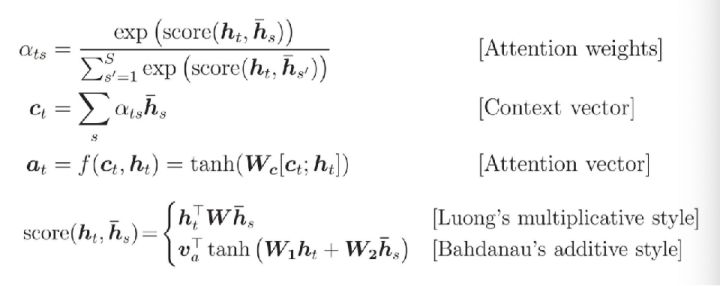
class BahdanauAttention(tf.keras.Model):
    def __init__(self, units):
        super(BahdanauAttention, self).__init__()
        self.W1 = tf.keras.layers.Dense(units)
        self.W2 = tf.keras.layers.Dense(units)
        self.V = tf.keras.layers.Dense(1)

    def call(self, features, hidden):
        hidden_with_time_axis = tf.expand_dims(hidden, 1)
        score = tf.nn.tanh(self.W1(features) + self.W2(hidden_with_time_axis))
        attention_weights = tf.nn.softmax(self.V(score), axis=1)
        context_vector = attention_weights * features
        context_vector = tf.reduce_sum(context_vector, axis=1)
        return context_vector, attention_weights

# 第三步是解码器, 基于seq2seq架构, 我们选取GRU作为解码器:

class RNN_Decoder(tf.keras.Model):
  def __init__(self, embedding_dim, units, vocab_size):
      super(RNN_Decoder, self).__init__()
      self.units = units
      self.embedding = tf.keras.layers.Embedding(vocab_size, embedding_dim)

      self.gru = tf.keras.layers.GRU(self.units, return_sequences=True,
                     return_state=True, recurrent_initializer=‘glorot_uniform')

      # 实例化两个全连接层
      self.fc1 = tf.keras.layers.Dense(self.units)
      self.fc2 = tf.keras.layers.Dense(vocab_size)
      # 实例化注意力机制
      self.attention = BahdanauAttention(self.units)
def call(self, x, features, hidden):
      # 首先使用注意力计算规则获得features和hidden的注意力结果
      context_vector, attention_weights = self.attention(features, hidden)
      x = self.embedding(x)
      x = tf.concat([tf.expand_dims(context_vector, 1), x], axis=-1)

      output, state = self.gru(x)
      x = self.fc1(output)

      x = tf.reshape(x, (-1, x.shape[2]))
      x = self.fc2(x)

      # 返回解码结果, gru隐层状态, 和注意力权重
      return x, state, attention_weights
# 开启一个用于梯度记录的上下文管理器
with tf.GradientTape() as tape:
        # 使用编码器处理输入的图片张量
        features = encoder(img_tensor)
        # 开始使用解码器循环解码,解码长度为target.shape[1]即文本描述张量的最大长度
        for i in range(1, target.shape[1]):
              # 使用解码器获得第一个预测值和隐含张量
              predictions, hidden, _ = decoder(dec_input, features, hidden)
              # 计算该解码过程的损失
              loss += loss_function(target[:, i], predictions)
              # 接下来这里使用了teacher_forcing来定义下一次解码的输入
              # 关于teacher_forcing请查看下方定义和作用
              dec_input = tf.expand_dims(target[:, i], 1)
# 全部循环解码完成后, 计算句子粒度的平均损失
average_loss = (loss / int(target.shape[1]))

# 获得整个模型训练的参数变量
trainable_variables = encoder.trainable_variables + decoder.trainable_variables

# 使用梯度管理器对象对参数变量求解梯度
gradients = tape.gradient(loss, trainable_variables)
    
# 根据梯度更新参数
optimizer.apply_gradients(zip(gradients, trainable_variables))

# 返回句子粒度的平均损失
return average_loss
# 使用编码器对图片进行编码
features = encoder(img_tensor_val)
dec_input = tf.expand_dims([tokenizer.word_index['<start>']], 0)
result = []
# 根据解码器结果生成最终的文本结果 
for i in range(max_length):  
      predictions, hidden, attention_weights = decoder(dec_input, features, hidden)
      predicted_id = tf.random.categorical(predictions, 1)[0][0].numpy()
      # 根据数值映射器和predicted_id获得对应单词(文本)并装入结果列表中
      result.append(tokenizer.index_word[predicted_id])
      if tokenizer.index_word[predicted_id] == '<end>':
            return result, attention_plot
      # 如果不是终止符, 则将本次的结果扩展维度作为下次解码器的输出
      dec_input = tf.expand_dims([predicted_id], 0)

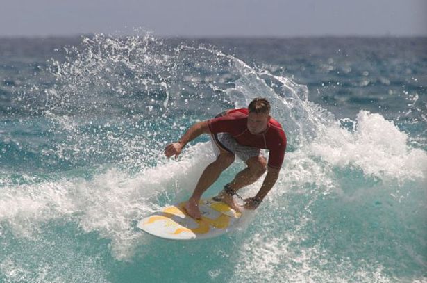
Prediction Caption: a person is sitting down to surfboard in no to their surf <end>