自动驾驶算法详解(3): LQR算法进行轨迹跟踪,lqr_speed_steering_control( )的python实现
前言:LQR算法在自动驾驶应用中,一般用在NOP、TJA、LCC这些算法的横向控制中,一般与曲率的前馈控制一起使用,来实现轨迹跟踪的目标,通过控制方向盘转角来实现横向控制。本文将使用python来实现 lqr_speed_steering_control( ) 轨迹跟踪算法的demo,通过同时控制转角与加速度来实现轨迹跟踪。如果对自动驾驶规划、控制、apollo算法细节、感知融合算法感兴趣,可以关
前言:
LQR算法在自动驾驶应用中,一般用在NOP、TJA、LCC这些算法的横向控制中,一般与曲率的前馈控制一起使用,来实现轨迹跟踪的目标,通过控制方向盘转角来实现横向控制。
本文将使用python来实现 lqr_speed_steering_control( ) 轨迹跟踪算法的demo,通过同时控制转角与加速度来实现轨迹跟踪。
如果对自动驾驶规划、控制、apollo算法细节、感知融合算法感兴趣,可以关注我的主页:
最新免费文章推荐:
prescan联合simulink进行FCW的仿真_自动驾驶 Player的博客-CSDN博客
Apollo Planning决策规划代码详细解析 (1):Scenario选择
自动驾驶算法详解 (1) : Apollo路径规划 Piecewise Jerk Path Optimizer的python实现
自动驾驶算法详解(5): 贝塞尔曲线进行路径规划的python实现
使用Vscode断点调试apollo的方法_自动驾驶 Player的博客-CSDN博客
Apollo规划决策算法仿真调试(1): 使用Vscode断点调试apollo的方法
Apollo规划决策算法仿真调试(4):动态障碍物绕行_自动驾驶 Player的博客-CSDN博客
正文如下:
一、LQR问题模型建立:
理论部分比较成熟,这里只介绍demo所使用的建模方程:
使用离散代数黎卡提方程求解
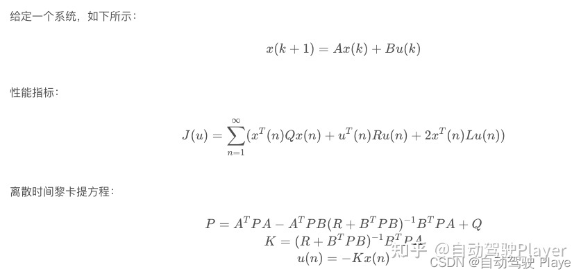

LQR控制的步骤:
选择参数矩阵Q,R
求解Riccati方程得到矩阵P
根据P计算 K = R − 1 B T P K=R^{-1}B^{T}P K=R−1BTP
计算控制量 u = − K x u=-Kx u=−Kx
系统状态矩阵:
 输入矩阵:
输入矩阵:

A矩阵:
B矩阵:

二、代码实现
# 导入相关包

import math

import sys

import os

import matplotlib.pyplot as plt

import numpy as np

import scipy.linalg as la


# cubic_spline_planner为自己实现的三次样条插值方法

try:

    from cubic_spline_planner import *

except ImportError:

    raise
设置轨迹途经点并生成轨迹:
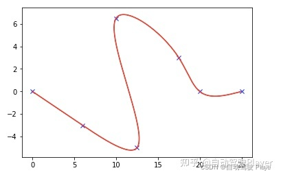
# 设置轨迹会经过的点

ax = [0.0, 6.0, 12.5, 10.0, 17.5, 20.0, 25.0]

ay = [0.0, -3.0, -5.0, 6.5, 3.0, 0.0, 0.0]

goal = [ax[-1], ay[-1]]


# 使用三次样条插值方法,根据途经点生成轨迹,x、y、yaw、曲率k,距离s

cx, cy, cyaw, ck, s = calc_spline_course(

        ax, ay, ds=0.1)


# 绘制规划好的轨迹

plt.plot(ax, ay, "xb", label="waypoints")

plt.plot(cx, cy, "-r", label="target course")
生成的轨迹如下:
设置期望速度:
# 设置目标速度

target_speed = 10.0 / 3.6  # simulation parameter km/h -> m/s


speed_profile = [target_speed] * len(cyaw)


direction = 1.0


# 转弯幅度较大时将速度设置为0,并将速度方向翻转

# Set stop point

for i in range(len(cyaw) - 1):

    dyaw = abs(cyaw[i + 1] - cyaw[i])

    switch = math.pi / 4.0 <= dyaw < math.pi / 2.0


    if switch:

        direction *= -1


    if direction != 1.0:

        speed_profile[i] = - target_speed

    else:

        speed_profile[i] = target_speed


    if switch:

        speed_profile[i] = 0.0


# 靠近目的地时,速度降低

# speed down

for i in range(40):

    speed_profile[-i] = target_speed / (50 - i)

    if speed_profile[-i] <= 1.0 / 3.6:

        speed_profile[-i] = 1.0 / 3.6


plt.plot(speed_profile, "-b", label="speed_profile")
期望速度如下:

定义求解所需要的数据结构与方法:
# 定义LQR 计算所需要的数据结构,以及DLQR的求解方法


# State 对象表示自车的状态,位置x、y,以及横摆角yaw、速度v

class State:


    def __init__(self, x=0.0, y=0.0, yaw=0.0, v=0.0):

        self.x = x

        self.y = y

        self.yaw = yaw

        self.v = v


# 更新自车的状态,采样时间足够小,则认为这段时间内速度相同,加速度相同,使用匀速模型更新位置

def update(state, a, delta):


    if delta >= max_steer:

        delta = max_steer

    if delta <= - max_steer:

        delta = - max_steer


    state.x = state.x + state.v * math.cos(state.yaw) * dt

    state.y = state.y + state.v * math.sin(state.yaw) * dt

    state.yaw = state.yaw + state.v / L * math.tan(delta) * dt

    state.v = state.v + a * dt


    return state


def pi_2_pi(angle):

    return (angle + math.pi) % (2 * math.pi) - math.pi


# 实现离散Riccati equation 的求解方法

def solve_dare(A, B, Q, R):

    """

    solve a discrete time_Algebraic Riccati equation (DARE)

    """

    x = Q

    x_next = Q

    max_iter = 150

    eps = 0.01


    for i in range(max_iter):

        x_next = A.T @ x @ A - A.T @ x @ B @ \

                la.inv(R + B.T @ x @ B) @ B.T @ x @ A + Q

        if (abs(x_next - x)).max() < eps:

            break

        x = x_next


    return x_next


# 返回值K 即为LQR 问题求解方法中系数K的解

def dlqr(A, B, Q, R):

    """Solve the discrete time lqr controller.

    x[k+1] = A x[k] + B u[k]

    cost = sum x[k].T*Q*x[k] + u[k].T*R*u[k]

    # ref Bertsekas, p.151

    """


    # first, try to solve the ricatti equation

    X = solve_dare(A, B, Q, R)


    # compute the LQR gain

    K = la.inv(B.T @ X @ B + R) @ (B.T @ X @ A)


    eig_result = la.eig(A - B @ K)


    return K, X, eig_result[0]


# 计算距离自车当前位置最近的参考点

def calc_nearest_index(state, cx, cy, cyaw):

    dx = [state.x - icx for icx in cx]

    dy = [state.y - icy for icy in cy]


    d = [idx ** 2 + idy ** 2 for (idx, idy) in zip(dx, dy)]


    mind = min(d)


    ind = d.index(mind)


    mind = math.sqrt(mind)


    dxl = cx[ind] - state.x

    dyl = cy[ind] - state.y


    angle = pi_2_pi(cyaw[ind] - math.atan2(dyl, dxl))

    if angle < 0:

        mind *= -1


    return ind, mind
设置起点参数:
# 设置起点的参数

T = 500.0  # max simulation time

goal_dis = 0.3

stop_speed = 0.05


state = State(x=-0.0, y=-0.0, yaw=0.0, v=0.0)


time = 0.0

x = [state.x]

y = [state.y]

yaw = [state.yaw]

v = [state.v]

t = [0.0]


pe, pth_e = 0.0, 0.0
使用LQR算法计算轨迹跟踪需要的加速度与前轮转角:
# 配置LQR 的参数
# === Parameters =====
# LQR parameter
lqr_Q = np.eye(5)
lqr_R = np.eye(2)
dt = 0.1 # time tick[s],采样时间
L = 0.5 # Wheel base of the vehicle [m],车辆轴距
max_steer = np.deg2rad(45.0) # maximum steering angle[rad]
show_animation = True
while T >= time:
ind, e = calc_nearest_index(state, cx, cy, cyaw)
sp = speed_profile
tv = sp[ind]
k = ck[ind]
v_state = state.v
th_e = pi_2_pi(state.yaw - cyaw[ind])
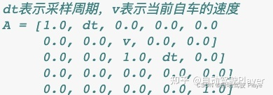
# 构建LQR表达式,X(k+1) = A * X(k) + B * u(k), 使用Riccati equation 求解LQR问题
# dt表示采样周期,v表示当前自车的速度
# A = [1.0, dt, 0.0, 0.0, 0.0
# 0.0, 0.0, v, 0.0, 0.0]
# 0.0, 0.0, 1.0, dt, 0.0]
# 0.0, 0.0, 0.0, 0.0, 0.0]
# 0.0, 0.0, 0.0, 0.0, 1.0]
A = np.zeros((5, 5))
A[0, 0] = 1.0
A[0, 1] = dt
A[1, 2] = v_state
A[2, 2] = 1.0
A[2, 3] = dt
A[4, 4] = 1.0
# 构建B矩阵,L是自车的轴距
# B = [0.0, 0.0
# 0.0, 0.0
# 0.0, 0.0
# v/L, 0.0
# 0.0, dt]
B = np.zeros((5, 2))
B[3, 0] = v_state / L
B[4, 1] = dt
K, _, _ = dlqr(A, B, lqr_Q, lqr_R)
# state vector,构建状态矩阵
# x = [e, dot_e, th_e, dot_th_e, delta_v]
# e: lateral distance to the path, e是自车到轨迹的距离
# dot_e: derivative of e, dot_e是自车到轨迹的距离的变化率
# th_e: angle difference to the path, th_e是自车与期望轨迹的角度偏差
# dot_th_e: derivative of th_e, dot_th_e是自车与期望轨迹的角度偏差的变化率
# delta_v: difference between current speed and target speed,delta_v是当前车速与期望车速的偏差
X = np.zeros((5, 1))
X[0, 0] = e
X[1, 0] = (e - pe) / dt
X[2, 0] = th_e
X[3, 0] = (th_e - pth_e) / dt
X[4, 0] = v_state - tv
# input vector,构建输入矩阵u
# u = [delta, accel]
# delta: steering angle,前轮转角
# accel: acceleration,自车加速度
ustar = -K @ X
# calc steering input
ff = math.atan2(L * k, 1) # feedforward steering angle
fb = pi_2_pi(ustar[0, 0]) # feedback steering angle
delta = ff + fb
# calc accel input
accel = ustar[1, 0]
dl, target_ind, pe, pth_e, ai = delta, ind, e, th_e, accel
state = update(state, ai, dl)
if abs(state.v) <= stop_speed:
target_ind += 1
time = time + dt
# check goal
dx = state.x - goal[0]
dy = state.y - goal[1]
if math.hypot(dx, dy) <= goal_dis:
print("Goal")
break
x.append(state.x)
y.append(state.y)
yaw.append(state.yaw)
v.append(state.v)
t.append(time)
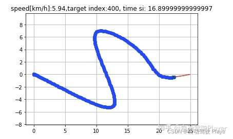
if target_ind % 100 == 0 and show_animation:
plt.cla()
# for stopping simulation with the esc key.
plt.gcf().canvas.mpl_connect('key_release_event',
lambda event: [exit(0) if event.key == 'escape' else None])
plt.plot(cx, cy, "-r", label="course")
plt.plot(x, y, "ob", label="trajectory")
plt.plot(cx[target_ind], cy[target_ind], "xg", label="target")
plt.axis("equal")
plt.grid(True)
plt.title("speed[km/h]:" + str(round(state.v * 3.6, 2))
+ ",target index:" + str(target_ind) + ", time si: " + str(time))
plt.pause(0.1)结果可视化:
if show_animation:  # pragma: no cover

        plt.close()

        plt.subplots(1)

        plt.plot(ax, ay, "xb", label="waypoints")

        plt.plot(cx, cy, "-r", label="target course")

        plt.plot(x, y, "-g", label="tracking")

        plt.grid(True)

        plt.axis("equal")

        plt.xlabel("x[m]")

        plt.ylabel("y[m]")

        plt.legend()


        plt.subplots(1)

        plt.plot(s, [np.rad2deg(iyaw) for iyaw in cyaw], "-r", label="yaw")

        plt.grid(True)

        plt.legend()

        plt.xlabel("line length[m]")

        plt.ylabel("yaw angle[deg]")


        plt.subplots(1)

        plt.plot(s, ck, "-r", label="curvature")

        plt.grid(True)

        plt.legend()

        plt.xlabel("line length[m]")

        plt.ylabel("curvature [1/m]")


        plt.show()
轨迹跟踪结果:
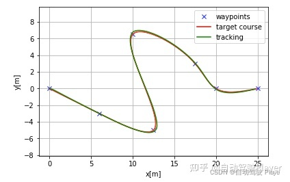
三、结果分析
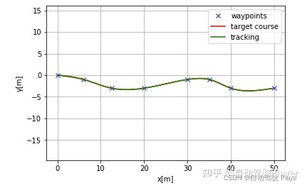
LQR算法一般用在NOP、TJA、LCC这些功能的横向控制,几种典型工况的轨迹跟踪效果如下:
1、正常变道工况
2、转弯工况

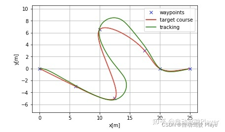
3、轴距对控制效果的影响
L = 0.5

L = 2.5

为开发者提供自动驾驶技术分享交流、实践成长、工具资源等,帮助开发者快速掌握自动驾驶技术。
更多推荐
 13
13 0
0- 0


 已为社区贡献4条内容

所有评论(0)