
CIC-IDS2017数据集训练和测试
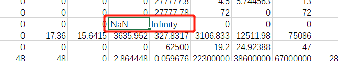
1、数据集预处理1.1整合数据并剔除脏数据如上图所示,整个数据集是分开的,想要训练,必须要整合在一起,同时在数据集中存在Nan和Infiniti脏数据(只有第15列和第16列存在)需要剔除:具体代码如下:```pythonimportpandasaspd#按行合并多个Dataframe数据defmergeData():monday=writeData("data\MachineLearningCV
1、数据集预处理
1.1 整合数据并剔除脏数据
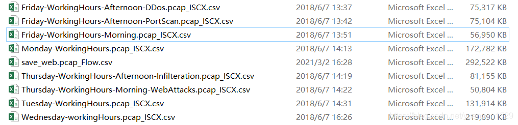
如上图所示,整个数据集是分开的,想要训练,必须要整合在一起,同时在数据集中存在 Nan 和 Infiniti 脏数据(只有第 15 列和第 16 列存在)需要剔除:
具体代码如下:
import pandas as pd

# 按行合并多个Dataframe数据
def mergeData():
    monday = writeData("data\MachineLearningCVE\Monday-WorkingHours.pcap_ISCX.csv")

    # 剔除第一行属性特征名称
    monday = monday.drop([0])
    friday1 = writeData("data\MachineLearningCVE\Friday-WorkingHours-Afternoon-DDos.pcap_ISCX.csv")
    friday1 = friday1.drop([0])
    friday2 = writeData("data\MachineLearningCVE\Friday-WorkingHours-Afternoon-PortScan.pcap_ISCX.csv")
    friday2 = friday2.drop([0])
    friday3 = writeData("data\MachineLearningCVE\Friday-WorkingHours-Morning.pcap_ISCX.csv")
    friday3 = friday3.drop([0])
    thursday1 = writeData("data\MachineLearningCVE\Thursday-WorkingHours-Afternoon-Infilteration.pcap_ISCX.csv")
    thursday1 = thursday1.drop([0])
    thursday2 = writeData("data\MachineLearningCVE\Thursday-WorkingHours-Morning-WebAttacks.pcap_ISCX.csv")
    thursday2 = thursday2.drop([0])
    tuesday = writeData("data\MachineLearningCVE\Tuesday-WorkingHours.pcap_ISCX.csv")
    tuesday = tuesday.drop([0])
    wednesday = writeData("data\MachineLearningCVE\Wednesday-workingHours.pcap_ISCX.csv")
    wednesday = wednesday.drop([0])
    frame = [monday,friday1,friday2,friday3,thursday1,thursday2,tuesday,wednesday]

    # 合并数据
    result = pd.concat(frame)
    list = clearDirtyData(result)
    result = result.drop(list)
    return result


# 清除CIC-IDS数据集中的脏数据,第一行特征名称和含有Nan、Infiniti等数据的行数
def clearDirtyData(df):
    dropList = df[(df[14]=="Nan")|(df[15]=="Infinity")].index.tolist()
    return dropList

raw_data=mergeData()
file = 'data/total.csv'
raw_data.to_csv(file, index=False, header=False)
将合并文件保存为 total.csv,省去每次训练都要重复操作的步骤
1.2 分析数据
在 panda 库中,dataframe 类型有一个很好用的函数 value_counts,可以用来统计标签数量,加载 total.csv 得到 raw_data,运行下面代码:
# 得到标签列索引
last_column_index = raw_data.shape[1] - 1
print(raw_data[last_column_index].value_counts())
打印结果如下:

由上图可以看到,整个数据集相当不平衡,正常数据非常大,而攻击流量却相当少,可以说整个数据集是相当不平衡的,怎么解决这个问题,下一节来说一说。
1.3 平衡数据集
针对这种情况,一般而言,是要扩充小的攻击数据集,其扩充方法有很多:
- 从数据源头采集更多数据
- 复制原有数据并加上随机噪声
- 重采样
- 根据当前数据集估计数据分布参数,使用该分布产生更多数据等
上面的方法都不太好整:
- 数据源头不用想了;
- 复制数据加上加上随机噪声,需要对于数据本身比较理解,否则容易出现问题;
- 重采样,因为数据量很少,想要达到平衡必须百倍扩充数据,重采样只适用于扩充量不大的情况(个人见解)
- 根据分布产生更多数据,因为数据太少了(只有几十个),而且特征太多,估计出来的分布会十分不准确,而由此分布产生的数据则更加不准确了。
由于上述方法不好整,我只好用一个不算方法的方法去做:复制粘贴,将每个数据集扩充到 5000 条以上(其实本质上类似于重采样),具体代码如下:
import pandas as pd

# 根据file读取数据
def writeData(file):
    print("Loading raw data...")
    raw_data = pd.read_csv(file, header=None,low_memory=False)
    return raw_data


# 将大的数据集根据标签特征分为15类,存储到lists集合中
def separateData(raw_data):
    # dataframe数据转换为多维数组
    lists=raw_data.values.tolist()
    temp_lists=[]

    # 生成15个空的list集合,用来暂存生成的15种特征集
    for i in range(0,15):
        temp_lists.append([])

    # 得到raw_data的数据标签集合
    label_set = lookData(raw_data)

    # 将无序的数据标签集合转换为有序的list
    label_list = list(label_set)

    for i in range(0,len(lists)):
        # 得到所属标签的索引号
        data_index = label_list.index(lists[i][len(lists[0])-1])
        temp_lists[data_index].append(lists[i])
        if i%5000==0:
            print(i)
    saveData(temp_lists,'data/expendData/')
    return temp_lists


# 将lists分批保存到file文件路径下
def saveData(lists,file):
    label_set = lookData(raw_data)
    label_list = list(label_set)
    for i in range(0,len(lists)):
        save = pd.DataFrame(lists[i])
        file1 = file+label_list[i]+'.csv'
        save.to_csv(file1,index=False,header=False)

def lookData(raw_data):
    # 打印数据集的标签数据数量
    last_column_index = raw_data.shape[1] - 1
    print(raw_data[last_column_index].value_counts())

    # 取出数据集标签部分
    labels = raw_data.iloc[:, raw_data.shape[1] - 1:]

    # 多维数组转为以为数组
    labels = labels.values.ravel()
    label_set = set(labels)
    return label_set

# lists存储着15类数据集,将数据集数量少的扩充到至少不少于5000条,然后存储起来。
def expendData(lists):
    totall_list = []
    for i in range(0,len(lists)):
        while len(lists[i])<5000:
            lists[i].extend(lists[i])
        print(i)
        totall_list.extend(lists[i])
    saveData(lists,'data/expendData/')
    save = pd.DataFrame(totall_list)
    file = 'data/expendData/totall_extend.csv'
    save.to_csv(file, index=False, header=False)


file = 'data/clearData/total.csv'
raw_data = writeData(file)
lists = separateData(raw_data)
expendData(lists)
再来看一下数据集的统计情况:

将这个数据集命名为 total_expend.csv,等使用的时候,我们仔细分析一下两个数据集对于模型训练到底有什么区别。
2、使用 sklearn 进行训练和测试
sklearn 分类算法有很多,这里以决策树为例。
2.1 数据处理
直接上代码吧:
import pandas as pd
import numpy as np
from sklearn.metrics import confusion_matrix, zero_one_loss
from sklearn.model_selection import train_test_split
import matplotlib.pyplot as plt
from sklearn import preprocessing

# 加载数据
raw_data_filename = "data/clearData/total_expend.csv"
print("Loading raw data...")
raw_data = pd.read_csv(raw_data_filename, header=None,low_memory=False)

# 随机抽取比例,当数据集比较大的时候,可以采用这个,可选项
raw_data=raw_data.sample(frac=0.03)

# 查看标签数据情况
last_column_index = raw_data.shape[1] - 1
print("print data labels:")
print(raw_data[last_column_index].value_counts())

# 将非数值型的数据转换为数值型数据
# print("Transforming data...")
raw_data[last_column_index], attacks = pd.factorize(raw_data[last_column_index], sort=True)

# 对原始数据进行切片,分离出特征和标签,第1~78列是特征,第79列是标签
features = raw_data.iloc[:, :raw_data.shape[1] - 1]  # pandas中的iloc切片是完全基于位置的索引
labels = raw_data.iloc[:, raw_data.shape[1] - 1:]

# 特征数据标准化,这一步是可选项
features = preprocessing.scale(features)
features = pd.DataFrame(features)

# 将多维的标签转为一维的数组
labels = labels.values.ravel()

# 将数据分为训练集和测试集,并打印维数
df = pd.DataFrame(features)
X_train, X_test, y_train, y_test = train_test_split(df, labels, train_size=0.8, test_size=0.2, stratify=labels)

# print("X_train,y_train:", X_train.shape, y_train.shape)
# print("X_test,y_test:", X_test.shape, y_test.shape)
上述大概流程可以分为:
- 加载数据
- 分析数据
- 非数值型数据转换数值数据
- 分离特征和标签
- 数据标准化\归一化\正则化
- 将这个数据集切分为训练集合测试集
2.2 训练和测试
import pandas as pd
import numpy as np
from sklearn.tree import DecisionTreeClassifier
from sklearn.metrics import confusion_matrix, zero_one_loss

# 训练模型
print("Training model...")
clf = DecisionTreeClassifier(criterion='entropy', max_depth=12, min_samples_leaf=1, splitter="best")
trained_model = clf.fit(X_train, y_train)
print("Score:", trained_model.score(X_train, y_train))

# 预测
print("Predicting...")
y_pred = clf.predict(X_test)
print("Computing performance metrics...")
results = confusion_matrix(y_test, y_pred)
error = zero_one_loss(y_test, y_pred)

# 根据混淆矩阵求预测精度
list_diag = np.diag(results)
list_raw_sum = np.sum(results, axis=1)
print("Predict accuracy of the decisionTree: ", np.mean(list_diag) / np.mean(list_raw_sum))
在 sklearn 中,训练模型和预测模型几乎是一个模板,想要换算法,只需要将上面的算法行替换即可,也就是:
clf = DecisionTreeClassifier(criterion='entropy', max_depth=12, min_samples_leaf=1, splitter="best")其他都可以不变
来看一下预测结果:
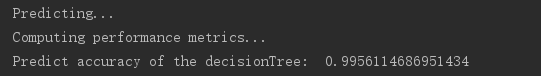
预测准确率为 99.56,算是很高了。
2.3 测试 total.csv 和 total_expend.csv 的区别
上面一节采用的数据集是 total.csv,也就是数据不平衡的数据集,但是从结果来看,其准确率很高,达到了 99.56%,然而,评价一个模型,准确率只是一个指标而已,我们来打印一下其混淆矩阵:

由上图可以看到,存在很多类别被误分的,但是为什么其准确率依然这么高呢?
这是因为数据不平衡,total.csv 数据集中,正常数据(也就是标签为 begin)的数据太多了,占据了几乎 99%的比例,只要它预测正确,那么整个数据集的准确率就会很高,至于其他标签的准确率哪怕再低,也不会有多大影响。
再来看看如果使用 total_expend.csv 数据集,先看准确率:
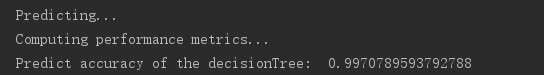
99.70%的准确率也很高,再看混淆矩阵打印:

可以看到,相比上面的,要好了很多,大部分类别都预测正确了(当然,这个也可能是因为类别标签大都重复造成的。)
绘制混淆矩阵代码:
class PlotConfusionMatrix:
    def plot_confusion_matrix(self,labels,cm, title='Confusion Matrix', cmap=plt.cm.binary):
        plt.imshow(cm, interpolation='nearest', cmap=cmap)
        plt.title(title)
        plt.colorbar()
        xlocations = np.array(range(len(labels)))
        plt.xticks(xlocations, labels, rotation=90)
        plt.yticks(xlocations, labels)
        plt.ylabel('True label')
        plt.xlabel('Predicted label')

    def prepareWork(self,labels, y_true, y_pred):
        tick_marks = np.array(range(len(labels))) + 0.5
        cm = confusion_matrix(y_true, y_pred)
        np.set_printoptions(precision=2)
        cm_normalized = cm.astype('float') / cm.sum(axis=1)[:, np.newaxis]
        plt.figure(figsize=(12, 8), dpi=120)

        ind_array = np.arange(len(labels))
        x, y = np.meshgrid(ind_array, ind_array)

        for x_val, y_val in zip(x.flatten(), y.flatten()):
            c = cm_normalized[y_val][x_val]
            if c > 0.01:
                plt.text(x_val, y_val, "%0.2f" % (c,), color='red', fontsize=7, va='center', ha='center')
        # offset the tick
        plt.gca().set_xticks(tick_marks, minor=True)
        plt.gca().set_yticks(tick_marks, minor=True)
        plt.gca().xaxis.set_ticks_position('none')
        plt.gca().yaxis.set_ticks_position('none')
        plt.grid(True, which='minor', linestyle='-')
        plt.gcf().subplots_adjust(bottom=0.15)

        self.plot_confusion_matrix(labels,cm_normalized, title='Normalized confusion matrix')
        # show confusion matrix
        # plt.savefig('image/confusion_matrix.png', format='png')
        plt.show()

# 绘制混淆矩阵
def plotMatrix(attacks, y_test, y_pred):
    # attacks是整个数据集的标签集合,但是切分测试集的时候,某些标签数量很少,可能会被去掉,这里要剔除掉这些标签
    y_test_set = set(y_test)
    y_test_list = list(y_test_set)
    attacks_test = []
    for i in range(0, len(y_test_set)):
        attacks_test.append(attacks[y_test_list[i]])
    p = PlotConfusionMatrix()
    p.prepareWork(attacks_test, y_test, y_pred)

# 绘制混淆矩阵图形,attacks是标签列表,y_test是测试结果,y_pred是预测结果
plotMatrix(attacks,y_test,y_pred)
2.4 调参
调参,就我所知有两种,一种是通过绘制学习曲线来调节某个超参数——横坐标为参数,纵坐标为准确度或者其他模型度量;另外一种是通过网格搜索交叉验证来调节多个超参数(本质是组合参数,然后循环验证)
2.4.1 绘制学习曲线调节决策树最优深度
参数那么多,如何确定最优的参数呢?针对一个参数调节的时候,可以画出学习曲线——横坐标为参数,纵坐标为准确度:
import matplotlib.pyplot as plt

test = []
for i in range(10):
    clf = tree.DecisionTreeClassifier(max_depth=i+1

                                    ,criterion="entropy"

                                    ,random_state=30

                                    ,splitter="random"

                                    )
    clf = clf.fit(Xtrain, Ytrain)
    score = clf.score(Xtest, Ytest)
    test.append(score)
plt.plot(range(1,11),test,color="red",label="max_depth")
plt.legend()
plt.show()
2.4.2 网格搜索寻找最优参数组合
#网格搜索:能够帮助我们同时调整多个参数的技术,枚举技术
import numpy as np

gini_thresholds = np.linspace(0,0.5,20)#基尼系数的边界
#entropy_thresholds = np.linespace(0, 1, 50)

#一串参数和这些参数对应的,我们希望网格搜索来搜索的参数的取值范围
parameters = {'splitter':('best','random')
              ,'criterion':("gini","entropy")
              ,"max_depth":[*range(1,10)]
              ,'min_samples_leaf':[*range(1,50,5)]
              ,'min_impurity_decrease':[*gini_thresholds]}

clf = DecisionTreeClassifier(random_state=25)#实例化决策树
GS = GridSearchCV(clf, parameters, cv=10)#实例化网格搜索,cv指的是交叉验证
GS.fit(Xtrain,Ytrain)
print(GS.best_params_)#从我们输入的参数和参数取值的列表中,返回最佳组合
print(GS.best_score_)#网格搜索后的模型的评判标准
旨在为数千万中国开发者提供一个无缝且高效的云端环境,以支持学习、使用和贡献开源项目。
更多推荐


 34
34 0
0- 0


 已为社区贡献5条内容

所有评论(0)