翻译自Tensorflow官方教程Neural machine translation with attention
声明：

• 本文将实现一个将西班牙语翻译成英语的seq2seq模型；
• 需要读者对seq2seq模型有了解；
• 需要读者对nlp中一些数据处理方式有了解；
• 翻译并非直译，会比原文更直白和丰富。
• 有些不重要的代码已通过（不重要）标记

我们准备训练一个seq2seq模型，将西班牙语翻译成英语。

在翻译中，原文本和翻译文本的词与词之间通常都有一定的对应关系。最理想的情况是：原文本的第$i$个词对应翻译文本的第$i$个词。当然大多数情况下不会有这么严格的对其关系。通过attention，我们可以得到如下图所示的混淆矩阵。

图中颜色鲜艳的部分表示横轴单词和纵轴单词关系密切，深蓝部分表示横轴单词和纵轴单词的关系疏远。这里的关系就是attention，显然，todavia pay more attention to you than at。

---

Note：下面的代码运行时间在10min左右，运行环境为单卡P100 GPU

code part 1: 导入需要的包（不重要）

from __future__ import absolute_import, division, print_function, unicode_literals

import tensorflow as tf

import matplotlib.pyplot as plt
import matplotlib.ticker as ticker
from sklearn.model_selection import train_test_split

import unicodedata
import re
import numpy as np
import os
import io
import time
复制

数据准备

数据介绍： 西班牙语到英语的翻译数据。
下载地址： http://www.manythings.org/anki/
数据示例： May I borrow this book? ¿Puedo tomar prestado este libro?

code part 2：下载数据集（不重要）

# Download the file
path_to_zip = tf.keras.utils.get_file(
    'spa-eng.zip', origin='http://storage.googleapis.com/download.tensorflow.org/data/spa-eng.zip',
    extract=True)

path_to_file = os.path.dirname(path_to_zip)+"/spa-eng/spa.txt"
复制

数据下载后，我们要做一些数据处理工作，包括一下4点：

1. 在每句话的首尾添加开始符和终止符；
2. 删除特殊符号；
3. 将文本型的单词转化成数值型的索引（也就是建立一个字典，可以完成word->id或者id->word的映射）；
4. padding每句话，使它们长度一致

code part 3: 数据处理（不重要）

# Converts the unicode file to ascii
def unicode_to_ascii(s):
  return ''.join(c for c in unicodedata.normalize('NFD', s)
      if unicodedata.category(c) != 'Mn')


def preprocess_sentence(w):
  w = unicode_to_ascii(w.lower().strip())

  # creating a space between a word and the punctuation following it
  # eg: "he is a boy." => "he is a boy ."
  # Reference:- https://stackoverflow.com/questions/3645931/python-padding-punctuation-with-white-spaces-keeping-punctuation
  w = re.sub(r"([?.!,¿])", r" \1 ", w)
  w = re.sub(r'[" "]+', " ", w)

  # replacing everything with space except (a-z, A-Z, ".", "?", "!", ",")
  w = re.sub(r"[^a-zA-Z?.!,¿]+", " ", w)

  w = w.rstrip().strip()

  # adding a start and an end token to the sentence
  # so that the model know when to start and stop predicting.
  w = '<start> ' + w + ' <end>'
  return w
复制

en_sentence = u"May I borrow this book?"
sp_sentence = u"¿Puedo tomar prestado este libro?"
print(preprocess_sentence(en_sentence))
print(preprocess_sentence(sp_sentence).encode('utf-8'))
复制

输出如下所示：
  <start> may i borrow this book ? <end>
  b'<start> \xc2\xbf puedo tomar prestado este libro ? <end>'

# 1. Remove the accents
# 2. Clean the sentences
# 3. Return word pairs in the format: [ENGLISH, SPANISH]
def create_dataset(path, num_examples):
  lines = io.open(path, encoding='UTF-8').read().strip().split('\n')

  word_pairs = [[preprocess_sentence(w) for w in l.split('\t')]  for l in lines[:num_examples]]

  return zip(*word_pairs)
复制

en, sp = create_dataset(path_to_file, None)
print(en[-1])
print(sp[-1])
复制

输出如下所示：
  <start> if you want to sound like a native speaker , you must be willing to practice saying the same sentence over and over in the same way that banjo players practice the same phrase over and over until they can play it correctly and at the desired tempo . <end>
  <start> si quieres sonar como un hablante nativo , debes estar dispuesto a practicar diciendo la misma frase una y otra vez de la misma manera en que un musico de banjo practica el mismo fraseo una y otra vez hasta que lo puedan tocar correctamente y en el tiempo esperado . <end>

def max_length(tensor):
  return max(len(t) for t in tensor)
复制

def tokenize(lang):
  lang_tokenizer = tf.keras.preprocessing.text.Tokenizer(
      filters='')
  lang_tokenizer.fit_on_texts(lang)

  tensor = lang_tokenizer.texts_to_sequences(lang)

  tensor = tf.keras.preprocessing.sequence.pad_sequences(tensor,
                                                         padding='post')

  return tensor, lang_tokenizer
复制

构造一个包含30000样本的数据集

code part 4：构造一个包含3000样本的数据集（不重要）

def load_dataset(path, num_examples=None):
  # creating cleaned input, output pairs
  targ_lang, inp_lang = create_dataset(path, num_examples)

  input_tensor, inp_lang_tokenizer = tokenize(inp_lang)
  target_tensor, targ_lang_tokenizer = tokenize(targ_lang)

  return input_tensor, target_tensor, inp_lang_tokenizer, targ_lang_tokenizer
复制

# Try experimenting with the size of that dataset
num_examples = 30000
input_tensor, target_tensor, inp_lang, targ_lang = load_dataset(path_to_file, num_examples)

# Calculate max_length of the target tensors
max_length_targ, max_length_inp = max_length(target_tensor), max_length(input_tensor)
复制

# Creating training and validation sets using an 80-20 split
input_tensor_train, input_tensor_val, target_tensor_train, target_tensor_val = train_test_split(input_tensor, target_tensor, test_size=0.2)

# Show length
print(len(input_tensor_train), len(target_tensor_train), len(input_tensor_val), len(target_tensor_val))
复制

输出如下所示：
  24000 24000 6000 6000

def convert(lang, tensor):
  for t in tensor:
    if t!=0:
      print ("%d ----> %s" % (t, lang.index_word[t]))
复制

print ("Input Language; index to word mapping")
convert(inp_lang, input_tensor_train[0])
print ()
print ("Target Language; index to word mapping")
convert(targ_lang, target_tensor_train[0])
复制

输出如下所示：
  Input Language; index to word mapping
  1 ----> <start>
  12 ----> me
  232 ----> duele
  9 ----> el
  644 ----> brazo
  3 ----> .
  2 ----> <end>

  Target Language; index to word mapping
  1 ----> <start>
  21 ----> my
  613 ----> arm
  551 ----> hurts
  3 ----> .
  2 ----> <end>

创建tf.data Dataset

code part 5：使用tf的dataset API将数据集包装起来

BUFFER_SIZE = len(input_tensor_train)
BATCH_SIZE = 64
steps_per_epoch = len(input_tensor_train)//BATCH_SIZE
embedding_dim = 256
units = 1024  # encoder层的hidden size
vocab_inp_size = len(inp_lang.word_index)+1
vocab_tar_size = len(targ_lang.word_index)+1

dataset = tf.data.Dataset.from_tensor_slices((input_tensor_train, target_tensor_train)).shuffle(BUFFER_SIZE)
dataset = dataset.batch(BATCH_SIZE, drop_remainder=True)
复制

example_input_batch, example_target_batch = next(iter(dataset))
example_input_batch.shape, example_target_batch.shape
复制

输出如下所示：
  (TensorShape([64, 16]), TensorShape([64, 11]))

encoder和decoder

seq2seq model有两部分组成：encoder和decoder。attention模块会被加载encoder的输出和decoder的隐藏状态之间，如下图所示。

传统的seq2seq是先将输入序列编码成一个encoder state，然后decode的时候，对每个target word，encoder state都不变。而seq2seq with attention使用attention vector代替encoder state。

attention vector可以看作一个target sentence到source sentence之间的关系矩阵。假设target sentence长度为3，source sentence长度为4，则这个关系矩阵的是3x4的矩阵。矩阵中每一行都是一个向量，向量的维度跟attention层隐藏层神经元的个数有关。


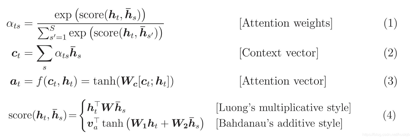
符号表示：
${\alpha }_{ts}$：target sentence和source sentence之间的attention值，通常，我们使用decoder的hidden state代替target sentence。shape=[batch_size]
$c_t$：上下文向量，shape=[batch_size, $s$]，$s$为encoder的隐藏层输出
$a_t$：attention vector，shape=[batch_size, $t$], 相当于每一个输出word都一个对应所有编码向量的attention，$t$为$W_c$的隐藏层输出
$v_a$：权重向量，将axis=2的维度reduce成1维，方便公式1的softmax
$h_t$：target sentence的隐藏层状态，shape=[batch_size, $s$]
${\bar{h}}_s$：source sentence的encoder输出，shape=[batch_size, source_sentence_size, $s$]
在公示4中有两种score函数可选，本文选择[Bahdanau's additive syle]。

下面我们用tensorflow的代码实现encoder，decoder和attention层。

code part 6: 实现encoder

class Encoder(tf.keras.Model):
  def __init__(self, vocab_size, embedding_dim, enc_units, batch_sz):
  	"""
  	:param vocab_size: int, vocabulary size, 字符词的个数，通常是word index的最大值+1
  	:param embedding_dim: int, embedding dimension, 嵌入词向量的维度
  	:param enc_units: int, GRU cell中神经元的个数
  	:parm batch_sz: int, batch size
  	"""
    super(Encoder, self).__init__()
    self.batch_sz = batch_sz  # batch size
    self.enc_units = enc_units  # encoder GRU's hidden size
    # embedding layer
    self.embedding = tf.keras.layers.Embedding(vocab_size, embedding_dim)
    # GRU layer
    self.gru = tf.keras.layers.GRU(self.enc_units,
                                   return_sequences=True,
                                   return_state=True,
                                   recurrent_initializer='glorot_uniform')

  def call(self, x, hidden):
    x = self.embedding(x)  # shape=[batch_size, timestep, embedding_size]
    # output shape = [batch_size, timestep, hidden_size]
    # state shape = [batch_size, hidden_size]
    output, state = self.gru(x, initial_state = hidden)
    return output, state

  def initialize_hidden_state(self):
  	"""
	initialize hidden state
	:return: state tensor, shape=[batch_size, hidden_size]
	"""
    return tf.zeros((self.batch_sz, self.enc_units))
复制

encoder = Encoder(vocab_inp_size, embedding_dim, units, BATCH_SIZE)

# sample input
sample_hidden = encoder.initialize_hidden_state()
sample_output, sample_hidden = encoder(example_input_batch, sample_hidden)
print ('Encoder output shape: (batch size, sequence length, units) {}'.format(sample_output.shape))
print ('Encoder Hidden state shape: (batch size, units) {}'.format(sample_hidden.shape))
复制

输出如下所示：
  Encoder output shape: (batch size, sequence length, units) (64, 16, 1024)
  Encoder Hidden state shape: (batch size, units) (64, 1024)
Encoder有两个输出，output和hidden state，分别对应前文的$h_s$和$h_t$。

code part 7: 实现attention

class BahdanauAttention(tf.keras.layers.Layer):
  def __init__(self, units):
  	"""
  	:param units: int, attention层神经元的个数，通常units大于1
  	"""
    super(BahdanauAttention, self).__init__()
    self.W1 = tf.keras.layers.Dense(units)
    self.W2 = tf.keras.layers.Dense(units)
    self.V = tf.keras.layers.Dense(1)

  def call(self, query, values):
    # hidden shape == (batch_size, hidden size)
    # hidden_with_time_axis shape == (batch_size, 1, hidden size)
    # we are doing this to perform addition to calculate the score
    hidden_with_time_axis = tf.expand_dims(query, 1)

    # score shape == (batch_size, max_length, 1)
    # we get 1 at the last axis because we are applying score to self.V
    # the shape of the tensor before applying self.V is (batch_size, max_length, units)
    score = self.V(tf.nn.tanh(
        self.W1(values) + self.W2(hidden_with_time_axis)))

    # attention_weights shape == (batch_size, max_length, 1)
    attention_weights = tf.nn.softmax(score, axis=1)

    # context_vector shape after sum == (batch_size, hidden_size)
    context_vector = attention_weights * values
    context_vector = tf.reduce_sum(context_vector, axis=1)

    return context_vector, attention_weights
复制

attention_layer = BahdanauAttention(10)
attention_result, attention_weights = attention_layer(sample_hidden, sample_output)

print("Attention result shape: (batch size, units) {}".format(attention_result.shape))
print("Attention weights shape: (batch_size, sequence_length, 1) {}".format(attention_weights.shape))
复制

输出如下所示：
  Attention result shape: (batch size, units) (64, 1024)
  Attention weights shape: (batch_size, sequence_length, 1) (64, 16, 1)

code part 8：实现decoder

class Decoder(tf.keras.Model):
  def __init__(self, vocab_size, embedding_dim, dec_units, batch_sz):
  	"""
  	:param vocab_size: int, 词表大小
  	:param embedding_dim: int, 嵌入词向量的维度，本文取值为256
  	:param dec_units: int, decoder GRU's hidden size
  	:param batch_sz: int, batch size
  	"""
    super(Decoder, self).__init__()
    self.batch_sz = batch_sz
    self.dec_units = dec_units
    self.embedding = tf.keras.layers.Embedding(vocab_size, embedding_dim)
    self.gru = tf.keras.layers.GRU(self.dec_units,
                                   return_sequences=True,
                                   return_state=True,
                                   recurrent_initializer='glorot_uniform')
    self.fc = tf.keras.layers.Dense(vocab_size)

    # used for attention
    self.attention = BahdanauAttention(self.dec_units)

  def call(self, x, hidden, enc_output):
    # enc_output shape == (batch_size, max_length, hidden_size)
    context_vector, attention_weights = self.attention(hidden, enc_output)

    # x shape after passing through embedding == (batch_size, 1, embedding_dim)
    x = self.embedding(x)

    # x shape after concatenation == (batch_size, 1, embedding_dim + hidden_size)
    # 本文中，embedding_dim=256, hidden_size=1024
    x = tf.concat([tf.expand_dims(context_vector, 1), x], axis=-1)

    # passing the concatenated vector to the GRU
    output, state = self.gru(x)

    # output shape == (batch_size * 1, hidden_size)
    output = tf.reshape(output, (-1, output.shape[2]))

    # output shape == (batch_size, vocab)
    x = self.fc(output)

    return x, state, attention_weights
复制

decoder = Decoder(vocab_tar_size, embedding_dim, units, BATCH_SIZE)

sample_decoder_output, _, _ = decoder(tf.random.uniform((BATCH_SIZE, 1)),
                                      sample_hidden, sample_output)

print ('Decoder output shape: (batch_size, vocab size) {}'.format(sample_decoder_output.shape))
复制

输出如下所示：
  Decoder output shape: (batch_size, vocab size) (64, 4935)

注意这里decoder的输入x的timestep=1，因为我们要采用teacher force的学习方式。另外，x的初始化方式也很特别，要知道0是padding value，1是开始符号的index，而这里decoder的初始输入是0到1之间的均匀分布，应该是一个不错的trick。

定义optimizer和损失函数

code part 9: 实现损失函数

optimizer = tf.keras.optimizers.Adam()
loss_object = tf.keras.losses.SparseCategoricalCrossentropy(
    from_logits=True, reduction='none')

def loss_function(real, pred):
  mask = tf.math.logical_not(tf.math.equal(real, 0))
  loss_ = loss_object(real, pred)

  mask = tf.cast(mask, dtype=loss_.dtype)
  loss_ *= mask

  return tf.reduce_mean(loss_)
复制

保存模型的checkpoint

code part 10: 定义checkpoint

checkpoint_dir = './training_checkpoints'
checkpoint_prefix = os.path.join(checkpoint_dir, "ckpt")
checkpoint = tf.train.Checkpoint(optimizer=optimizer,
                                 encoder=encoder,
                                 decoder=decoder)
复制

训练

训练的方式teacher force方式。即：预测target sentence的每个word时，使用上一步的word的真实值。关于teacher force的细节可以看：What is Teacher Forcing for Recurrent Neural Networks?。与teacher force相对应的就是：使用上一步word的预测值，预测下一个word。

训练过程如下：

1. encoder以source sentence为输入，输出编码后的输出和状态。
2. decoder以编码输出、编码状态、decoder上一步的word真实值为输入。
3. decoder输出预测word和解码状态
4. 使用新预测的解码状态，使用teacher force的方式解码下一个word。
5. 反向传播和梯度计算。

code part 11: 定义训练过程

@tf.function
def train_step(inp, targ, enc_hidden):
  """
  :param inp: tensor, 输入的source sentence
  :param targ: tensor, 输入的target sentence
  :param enc_hidden: tensor, 初始化的encoder hidden state
  """
  loss = 0

  with tf.GradientTape() as tape:
    enc_output, enc_hidden = encoder(inp, enc_hidden)

    dec_hidden = enc_hidden

    dec_input = tf.expand_dims([targ_lang.word_index['<start>']] * BATCH_SIZE, 1)

    # Teacher forcing - feeding the target as the next input
    for t in range(1, targ.shape[1]):
      # passing enc_output to the decoder
      predictions, dec_hidden, _ = decoder(dec_input, dec_hidden, enc_output)

      loss += loss_function(targ[:, t], predictions)

      # using teacher forcing
      dec_input = tf.expand_dims(targ[:, t], 1)

  batch_loss = (loss / int(targ.shape[1]))

  variables = encoder.trainable_variables + decoder.trainable_variables

  gradients = tape.gradient(loss, variables)

  optimizer.apply_gradients(zip(gradients, variables))

  return batch_loss
复制

code part 12: 开始训练

EPOCHS = 10

for epoch in range(EPOCHS):
  start = time.time()

  enc_hidden = encoder.initialize_hidden_state()
  total_loss = 0

  for (batch, (inp, targ)) in enumerate(dataset.take(steps_per_epoch)):
    batch_loss = train_step(inp, targ, enc_hidden)
    total_loss += batch_loss

    if batch % 100 == 0:
      print('Epoch {} Batch {} Loss {:.4f}'.format(epoch + 1,
                                                   batch,
                                                   batch_loss.numpy()))
  # saving (checkpoint) the model every 2 epochs
  if (epoch + 1) % 2 == 0:
    checkpoint.save(file_prefix = checkpoint_prefix)

  print('Epoch {} Loss {:.4f}'.format(epoch + 1,
                                      total_loss / steps_per_epoch))
  print('Time taken for 1 epoch {} sec\n'.format(time.time() - start))
复制

输出如下所示：
  Epoch 1 Batch 0 Loss 4.5660
  Epoch 1 Batch 100 Loss 2.1718
  Epoch 1 Batch 200 Loss 1.8068
  Epoch 1 Batch 300 Loss 1.6708
  Epoch 1 Loss 2.0163
  Time taken for 1 epoch 26.63117527961731 sec
  Epoch 2 Batch 0 Loss 1.5327
  Epoch 2 Batch 100 Loss 1.4952
  Epoch 2 Batch 200 Loss 1.2592
  Epoch 2 Batch 300 Loss 1.2441
  Epoch 2 Loss 1.3629
  Time taken for 1 epoch 15.648634672164917 sec
  Epoch 3 Batch 0 Loss 1.2130
  Epoch 3 Batch 100 Loss 1.0544
  Epoch 3 Batch 200 Loss 0.8962
  Epoch 3 Batch 300 Loss 0.8810
  Epoch 3 Loss 0.9473
  Time taken for 1 epoch 15.271944046020508 sec
  Epoch 4 Batch 0 Loss 0.6253
  Epoch 4 Batch 100 Loss 0.6916
  Epoch 4 Batch 200 Loss 0.6733
  Epoch 4 Batch 300 Loss 0.6504
  Epoch 4 Loss 0.6386
  Time taken for 1 epoch 15.564900398254395 sec
  Epoch 5 Batch 0 Loss 0.4521
  Epoch 5 Batch 100 Loss 0.4017
  Epoch 5 Batch 200 Loss 0.3624
  Epoch 5 Batch 300 Loss 0.4475
  Epoch 5 Loss 0.4322
  Time taken for 1 epoch 15.272238969802856 sec
  Epoch 6 Batch 0 Loss 0.2982
  Epoch 6 Batch 100 Loss 0.2609
  Epoch 6 Batch 200 Loss 0.3089
  Epoch 6 Batch 300 Loss 0.2583
  Epoch 6 Loss 0.2987
  Time taken for 1 epoch 15.556654214859009 sec
  Epoch 7 Batch 0 Loss 0.2139
  Epoch 7 Batch 100 Loss 0.2213
  Epoch 7 Batch 200 Loss 0.1933
  Epoch 7 Batch 300 Loss 0.2394
  Epoch 7 Loss 0.2141
  Time taken for 1 epoch 15.23383378982544 sec
  Epoch 8 Batch 0 Loss 0.1232
  Epoch 8 Batch 100 Loss 0.1565
  Epoch 8 Batch 200 Loss 0.1201
  Epoch 8 Batch 300 Loss 0.1961
  Epoch 8 Loss 0.1604
  Time taken for 1 epoch 15.483410835266113 sec
  Epoch 9 Batch 0 Loss 0.1311
  Epoch 9 Batch 100 Loss 0.1043
  Epoch 9 Batch 200 Loss 0.1175
  Epoch 9 Batch 300 Loss 0.1734
  Epoch 9 Loss 0.1242
  Time taken for 1 epoch 15.270419836044312 sec
  Epoch 10 Batch 0 Loss 0.1079
  Epoch 10 Batch 100 Loss 0.0715
  Epoch 10 Batch 200 Loss 0.1141
  Epoch 10 Batch 300 Loss 0.1267
  Epoch 10 Loss 0.1009
  Time taken for 1 epoch 15.481101036071777 sec

预测

预测的过程和训练差不多，不同的地方在于，不实用teacher force方式。

code part 13: 定义推理过程

def evaluate(sentence):
  attention_plot = np.zeros((max_length_targ, max_length_inp))

  sentence = preprocess_sentence(sentence)

  inputs = [inp_lang.word_index[i] for i in sentence.split(' ')]
  inputs = tf.keras.preprocessing.sequence.pad_sequences([inputs],
                                                         maxlen=max_length_inp,
                                                         padding='post')
  inputs = tf.convert_to_tensor(inputs)

  result = ''

  hidden = [tf.zeros((1, units))]
  enc_out, enc_hidden = encoder(inputs, hidden)

  dec_hidden = enc_hidden
  dec_input = tf.expand_dims([targ_lang.word_index['<start>']], 0)

  for t in range(max_length_targ):
    predictions, dec_hidden, attention_weights = decoder(dec_input,
                                                         dec_hidden,
                                                         enc_out)

    # storing the attention weights to plot later on
    attention_weights = tf.reshape(attention_weights, (-1, ))
    attention_plot[t] = attention_weights.numpy()

    predicted_id = tf.argmax(predictions[0]).numpy()

    result += targ_lang.index_word[predicted_id] + ' '

    if targ_lang.index_word[predicted_id] == '<end>':
      return result, sentence, attention_plot

    # the predicted ID is fed back into the model
    dec_input = tf.expand_dims([predicted_id], 0)

  return result, sentence, attention_plot
复制

code part 14: 绘制attention混淆矩阵

# function for plotting the attention weights
def plot_attention(attention, sentence, predicted_sentence):
  fig = plt.figure(figsize=(10,10))
  ax = fig.add_subplot(1, 1, 1)
  ax.matshow(attention, cmap='viridis')

  fontdict = {'fontsize': 14}

  ax.set_xticklabels([''] + sentence, fontdict=fontdict, rotation=90)
  ax.set_yticklabels([''] + predicted_sentence, fontdict=fontdict)

  ax.xaxis.set_major_locator(ticker.MultipleLocator(1))
  ax.yaxis.set_major_locator(ticker.MultipleLocator(1))

  plt.show()
复制

code part 15: 翻译

def translate(sentence):
  result, sentence, attention_plot = evaluate(sentence)

  print('Input: %s' % (sentence))
  print('Predicted translation: {}'.format(result))

  attention_plot = attention_plot[:len(result.split(' ')), :len(sentence.split(' '))]
  plot_attention(attention_plot, sentence.split(' '), result.split(' '))
复制

模型加载和测试

# restoring the latest checkpoint in checkpoint_dir
checkpoint.restore(tf.train.latest_checkpoint(checkpoint_dir))
复制

输出如下所示：
  <tensorflow.python.training.tracking.util.CheckpointLoadStatus at 0x7fb2117fb908>

translate(u'hace mucho frio aqui.')
复制

输出如下所示：
  Input: <start> hace mucho frio aqui . <end>
  Predicted translation: it s very cold here . <end>

translate(u'esta es mi vida.')
复制

输出如下所示：
  Input: <start> esta es mi vida . <end>
  Predicted translation: this is my life . <end>