一、循环神经网络（RNN）

1、特点：RNN对具有序列特性的数据非常有效，它能够挖掘数据中的时序信息和语义信息，利用它的这种能力使得深度学习模型在语音识别、语言模型、机器翻译以及时序分析等NLP领域的问题使有所突破。

序列特性：符合时间顺序、逻辑顺序或者其它顺序，例如人类的自然语言，符合某种逻辑或规则的字词拼凑排列起来的；发出的声音，是通过每一帧每一帧衔接起来，才凑成所听到的话；股票，随着时间的推移，会产生具有顺序的一系列数字。这些都是具有序列特性的。

2、为什么需要RNN？
其他的神经网络都只能单独处理一个一个的输入，前一个输入和后一个输入是完全没有关系的。但是某些任务需要更好的处理序列信息，即前面的输入是和后面一个输入是有关系的。

eg， I like eating apple！

         The Apple is a great company

现在给apple打标签，都知道第一个apple意思是苹果，第二个Apple是特殊名词，苹果公司，假设我们已经有了标记好的数据来训练模型，当我们使用全连接神经网络时，用这个的apple的特征向量输入模型中，在输出正确结果时，让lable中的正确lable的概率最大来训练模型，但在语料库中，有的apple是水果，有的是苹果公司，这将导致，模型在训练过程中，预测的准确程度取决于训练集的哪个lable多一些，从而看来，这个模型没有任何作用。问题出现在我们没有结合上下文语义去训练模型，而是单独在训练apple这个单词的lable，这个就是全连接神经网络所不能做到的，于是我们就使用了RNN。

全连接网络结构

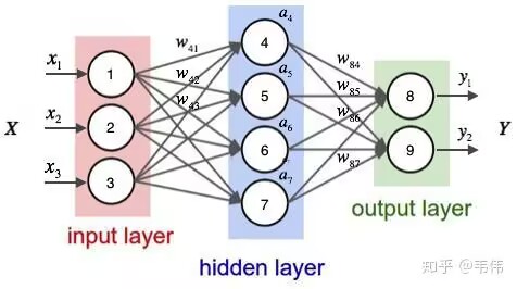
3、卷积神经网络与循环神经网络的简单对比

CNN：借助卷积核（kernel）提取特征后，送入后续网络（如Dense）进行分类、目标检测等操作。CNN借助卷积核从空间维度提取信息，卷积核参数空间共享。

RNN：借助循环核（cell）提取特征后，送入后续网络（如Dense）进行预测等操作。RNN借助循环核从时间维度提取信息，循环核参数时间共享。

4、RNN结构

（1）循环核

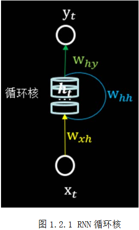
循环核具有记忆力，通过不同时刻的参数共享，实现了对时间序列的信息提取。每个循环核有多个记忆体，对应上图的多个小圆柱。记忆体内存储着每个时刻的状态信息，这里。其中、为权重矩阵，为偏置，为当前时刻的输入特征，为记忆体上一时刻存储的状态信息，tahn为激活函数。

当前时刻循环核的输出特征，其中为权重矩阵、为偏置、sofymax为激活函数，其实就相当于一层全连接层，当设定记忆体个数从而改变记忆容量，当记忆体个数被指定，输入输出维度被指定，周围这些待训练参数的维度也被限定了。在前向传播时，记忆体内存储的状态信息在每个时刻都被刷新，而三个参数和两个偏置项自始至终都是固定不变的。在反向传播 中，三个参数矩阵和两个偏置项由梯度下降法更新。

（2）循环核按时间步展开

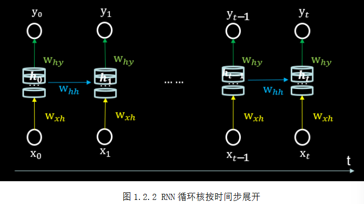
举个容易理解的例子，eg.I love you，使用RNN干这件事时，比如命名实体识别，代表I这个单词向量,代表love这个单词向量，代表you这一单词向量，以此类推.....

三个参数矩阵和两个偏置项都固定不变，我们训练优化的就是这些参数矩阵，训练完成后，使用效果最好的参数矩阵执行前向传播，然后输出预测结果，其实是和人类预测是一致的：我们脑中的记忆体每个时刻都根据当前的输入而更新，当前的预测推理是根据我们以往的知识积累用固化下来的“参数矩阵”进行的推理判断。

由此看出，循环神经网络就是借助循环核实现时间特征提取后把提取到的信息送入全连接网络，从而实现连续数据的预测。

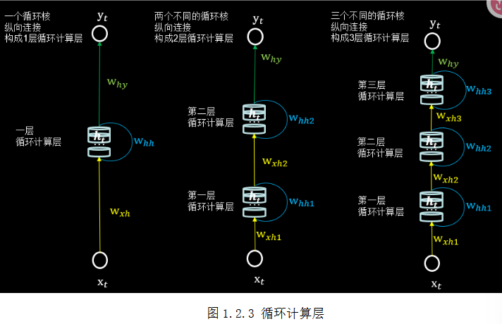
（3）循环计算层：向输出方向生长

在RNN中，每个循环核构成一层循环计算层，循环计算层的层数是向输出方向增长的。

（4）定义损失函数

RNN的损失函数与其它网络的区别在于：由于它每个时刻的节点都可能有一个输出，所以RNN 的总损失为所有时刻（或部分）上的损失和。

（5）Tensorflow语言描述循环计算层

tf.keras.layers.SimpleRNN(神经元个数，activation='激活函数'，return_sequences=是否每个时刻输出ht到下一层)

神经元个数：即循环核中记忆体的个数

return_sequences:在输出序列中，返回最后时间的输出值还是返回全部时间步的输出。False返回最后时刻的输出，True返回全部时刻。当下一层依然是RNN层，通常为True，反之如果后面是Dense层，通常为False。

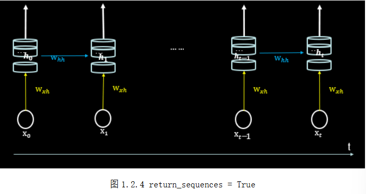
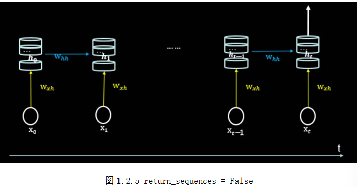
输入维度：三维张量（输入样本数，循环核时间展开步数，每个时间步输入特征个数）。

 根据上图中的左图看出，一共要送入RNN层两组数据，每组数据经过一个时间步就会得到输出结果，每个时间步送入三个数值，则输入循环层的数据维度就是[2,1,3]。右图输入只有一组数据，分四个时间步送入循环层，每个时间步送入两个数据，则输入循环层的数据维度是[1,4,2]。

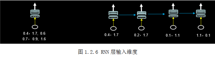
输出维度：当return_sequences=True,三维张量（输入样本数，循环核时间展开步数，本层的神经元个数），当等于False，二维张量（输入样本数，本层的神经元个数）

activation：‘激活函数’（不写就默认使用tanh）

eg.SimpleRNN(3,return_sequences=True),定义了一个具有三个记忆体的循环核，这个循环核会在每个时间步输出。

5、字母预测例子（1pre1）

（1）循环计算过程

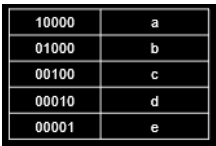
输入字母预测下一个字母——输入a预测出b、输入b预测出c、输入c预测出d、输入d预测出e

、输入e预测出a。计算机不认识字母，只认识数字，所以需要把字母进行编码。在这里假设使用独热编码（实际可以使用其他编码），编码结果如图

假设使用一层RNN网络，记忆体的个数选取3，则字母预测的网络如下图。

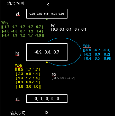
     假设输入字母b，即输入为[0,1,0,0,0]，这时上一时刻的记忆体状态信息为0。由上文理论知识得到： =  tanh([-2.3   0.8   1.1] + 0 + [0.5  0.3  -0.2])  =  tanh[-1.8   1.1   0.9]=[-0.9   0.8   0.7] ，这个过程可以理解为脑中记忆因为当前输入的事物而更新了。

     输出是把提取到的时间信息通过全连接进行识别预测的过程，是整个网络的输出层。=softmax（[-0.7   -0.6   2.9   0.7   -0.8]  + [0.0   0.1   0.4  -0.7   0.1] ）= softmax([-0.7   -0.5  3.3  0.0  -0.7]) = [0.02  0.02  0.91  0.03  0.02]。可见模型认为有91%的可能性输出字母c，所以循环网络输出了预测结果c。

（2）实践过程

a.用独热编码的方式实现：

按照六部法八股套路进行编码：

#  import相关模块
import numpy as np
import tensorflow as tf
from tensorflow.keras.layers import Dense, SimpleRNN
import matplotlib.pyplot as plt
import os
#  生成训练用的输入特征x_train和标签y_train(输入特征a对应的标签是b、输入的特征b对应的标签是c、依次类推)
input_word = "abcde"
w_to_id = {'a': 0, 'b': 1, 'c': 2, 'd': 3, 'e': 4}  # 单词映射到数值id的词典
id_to_onehot = {0: [1., 0., 0., 0., 0.], 1: [0., 1., 0., 0., 0.], 2: [0., 0., 1., 0., 0.], 3: [0., 0., 0., 1., 0.],
                4: [0., 0., 0., 0., 1.]}  # id编码为one-hot

x_train = [id_to_onehot[w_to_id['a']], id_to_onehot[w_to_id['b']], id_to_onehot[w_to_id['c']],
           id_to_onehot[w_to_id['d']], id_to_onehot[w_to_id['e']]]
y_train = [w_to_id['b'], w_to_id['c'], w_to_id['d'], w_to_id['e'], w_to_id['a']]

#  打乱顺序后变形成RNN输入需要的维度
np.random.seed(7)
np.random.shuffle(x_train)
np.random.seed(7)
np.random.shuffle(y_train)
tf.random.set_seed(7)

# 使x_train符合SimpleRNN输入要求：[送入样本数， 循环核时间展开步数， 每个时间步输入特征个数]。
# 此处整个数据集送入，送入样本数为len(x_train)；输入1个字母出结果，循环核时间展开步数为1; 表示为独热码有5个输入特征，每个时间步输入特征个数为5
x_train = np.reshape(x_train, (len(x_train), 1, 5))
y_train = np.array(y_train)
#  构建模型：一个具有3个记忆体的循环层+一层全连接---Compile-fit-summary
model = tf.keras.Sequential([
    SimpleRNN(3),   #  因为默认return_sequences = False
    Dense(5, activation='softmax')  #  全连接层，输出5个类别的概率分布
])

model.compile(optimizer=tf.keras.optimizers.Adam(0.01),
              loss=tf.keras.losses.SparseCategoricalCrossentropy(from_logits=False),
              metrics=['sparse_categorical_accuracy'])  #Adam学习率为0.01
#  断点训练
checkpoint_save_path = "./checkpoint/rnn_onehot_1pre1.ckpt"
if os.path.exists(checkpoint_save_path + '.index'):
    print('-------------load the model-----------------')
    model.load_weights(checkpoint_save_path)

cp_callback = tf.keras.callbacks.ModelCheckpoint(filepath=checkpoint_save_path,
                                                 save_weights_only=True,
                                                 save_best_only=True,
                                                 monitor='loss')  # 由于fit没有给出测试集，不计算测试集准确率，根据loss，保存最优模型

history = model.fit(x_train, y_train, batch_size=32, epochs=100, callbacks=[cp_callback])

model.summary()

# print(model.trainable_variables)
file = open('./weights.txt', 'w')  # 参数提取
for v in model.trainable_variables:
    file.write(str(v.name) + '\n')
    file.write(str(v.shape) + '\n')
    file.write(str(v.numpy()) + '\n')
file.close()

###############################################    show   ###############################################

# 显示训练集和验证集的acc和loss曲线
acc = history.history['sparse_categorical_accuracy']
loss = history.history['loss']

plt.subplot(1, 2, 1)
plt.plot(acc, label='Training Accuracy')
plt.title('Training Accuracy')
plt.legend()

plt.subplot(1, 2, 2)
plt.plot(loss, label='Training Loss')
plt.title('Training Loss')
plt.legend()
plt.show()

############### predict #############

preNum = int(input("input the number of test alphabet:"))
for i in range(preNum):
    alphabet1 = input("input test alphabet:")
    alphabet = [id_to_onehot[w_to_id[alphabet1]]]
    # 使alphabet符合SimpleRNN输入要求：[送入样本数， 循环核时间展开步数， 每个时间步输入特征个数]。此处验证效果送入了1个样本，送入样本数为1；输入1个字母出结果，所以循环核时间展开步数为1; 表示为独热码有5个输入特征，每个时间步输入特征个数为5
    alphabet = np.reshape(alphabet, (1, 1, 5))
    result = model.predict([alphabet])
    pred = tf.argmax(result, axis=1)
    pred = int(pred)
    tf.print(alphabet1 + '->' + input_word[pred])

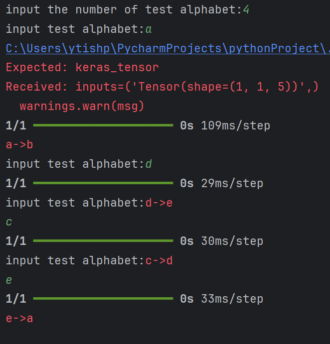
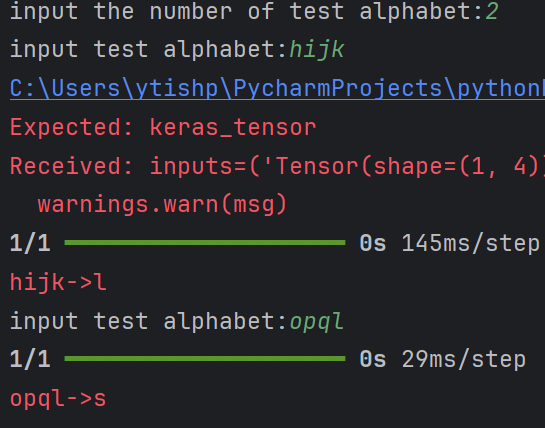
下图是预测的效果图，首先是输入需要执行预测任务的次数，随后等待驶入一个字母，将这个字母转换为独热码形式后调整为RNN层希望的形状，然后通过predict得到预测结果，选出预测结果中最大的一个即为预测结果。

b.用Embedding编码的方式实现：

为什么使用Embedding编码？

独热码：数据量大，过于稀疏，映射之间是独立的，没有表现出关联性。

Embedding编码：是一种单词编码方法，用于低维向量实现了编码。这种编码通过神经网络训练优化，能表达出单词间的相关性。

tensorflow2中的词向量空间编码层 ：

tf.keras.layers.Embedding(词汇表大小，编码维度)

词汇表大小：编码一共要表示多少个单词；
编码维度：用几个数字表达一个单词；

输入维度：二维张量[送入样本数，循环核时间展开步数]

输出维度：三维张量[送入样本数，循环核时间展开步数]

   eg.tf.keras.layers.Embedding(100,3)。对于数字1-100进行编码，词汇表大小就是100，每个自然数用三个数字表示，编码维度就是3，所以Embedding层的参数是100和3。比如数字[4]embedding为[0.25,  0.1,  0.11]。

  Embedding实现1pre1：

import numpy as np
import tensorflow as tf
from tensorflow.keras.layers import Dense, SimpleRNN, Embedding
import matplotlib.pyplot as plt
import os

input_word = "abcde"
w_to_id = {'a': 0, 'b': 1, 'c': 2, 'd': 3, 'e': 4}  # 单词映射到数值id的词典

#以下这个与独热编码不同的地方
x_train = [w_to_id['a'], w_to_id['b'], w_to_id['c'], w_to_id['d'], w_to_id['e']]
y_train = [w_to_id['b'], w_to_id['c'], w_to_id['d'], w_to_id['e'], w_to_id['a']]

np.random.seed(7)
np.random.shuffle(x_train)
np.random.seed(7)
np.random.shuffle(y_train)
tf.random.set_seed(7)

# 使x_train符合Embedding输入要求：[送入样本数， 循环核时间展开步数] ，
# 此处整个数据集送入所以送入，送入样本数为len(x_train)；输入1个字母出结果，循环核时间展开步数为1。
x_train = np.reshape(x_train, (len(x_train), 1))
y_train = np.array(y_train)

model = tf.keras.Sequential([
    Embedding(5, 2),  #  比独热编码形式多了一个Embedding层，对于输入数据进行编码，这一层会生成一个五行两列的可训练参数矩阵，实现编码可训练。
    SimpleRNN(3),
    Dense(5, activation='softmax')
])

model.compile(optimizer=tf.keras.optimizers.Adam(0.01),
              loss=tf.keras.losses.SparseCategoricalCrossentropy(from_logits=False),
              metrics=['sparse_categorical_accuracy'])

checkpoint_save_path = "./checkpoint/run_embedding_1pre1.ckpt"

if os.path.exists(checkpoint_save_path + '.index'):
    print('-------------load the model-----------------')
    model.load_weights(checkpoint_save_path)

cp_callback = tf.keras.callbacks.ModelCheckpoint(filepath=checkpoint_save_path,
                                                 save_weights_only=True,
                                                 save_best_only=True,
                                                 monitor='loss')  # 由于fit没有给出测试集，不计算测试集准确率，根据loss，保存最优模型

history = model.fit(x_train, y_train, batch_size=32, epochs=100, callbacks=[cp_callback])

model.summary()

# print(model.trainable_variables)
file = open('./weights.txt', 'w')  # 参数提取
for v in model.trainable_variables:
    file.write(str(v.name) + '\n')
    file.write(str(v.shape) + '\n')
    file.write(str(v.numpy()) + '\n')
file.close()

###############################################    show   ###############################################

# 显示训练集和验证集的acc和loss曲线
acc = history.history['sparse_categorical_accuracy']
loss = history.history['loss']

plt.subplot(1, 2, 1)
plt.plot(acc, label='Training Accuracy')
plt.title('Training Accuracy')
plt.legend()

plt.subplot(1, 2, 2)
plt.plot(loss, label='Training Loss')
plt.title('Training Loss')
plt.legend()
plt.show()

############### predict #############

preNum = int(input("input the number of test alphabet:"))
for i in range(preNum):
    alphabet1 = input("input test alphabet:")
    alphabet = [w_to_id[alphabet1]]
    # 使alphabet符合Embedding输入要求：[送入样本数， 循环核时间展开步数]。
    # 此处验证效果送入了1个样本，送入样本数为1；输入1个字母出结果，循环核时间展开步数为1。
    alphabet = np.reshape(alphabet, (1, 1))
    result = model.predict(alphabet)
    pred = tf.argmax(result, axis=1)
    pred = int(pred)
    tf.print(alphabet1 + '->' + input_word[pred])

只需要将读到的输入字母直接查找表示它的ID值，然后调整为Embedding层希望的形状输入网络进行预测即可。

6、字母预测例子（4pre1）

      1pre1是输入一个字母预测出下一个字母的例子，4pre1是连续输入多（这里取4）个字母预测下一个字母的例子。这里仍然使用三个记忆体，初始记忆体内的记忆为0。接下来用一套训练好的参数矩阵感受循环计算的前向传播过程，在这个过程中的每个时刻参数矩阵是固定，记忆体会在每个时刻被更新。下面以输入bcde预测a为例：

   在第一个时刻，b的独热码[0, 1, 0, 0, 0]输入，记忆体根据更新公式=tanh([-1.5   0.2   0.3] + 0 + [0.2  0.0  -0.1])  =  tanh[-1.3   0.2   0.2]=[-0.9   0.2   0.2]刷新。

   在第二个时刻，c的独热码[0, 0, 1, 0, 0]输入，记忆体根据更新公式 = tanh([-0.3   1.7   0.7] + [1.1, 1.1, 0.5] + [0.2  0.0  -0.1])  =  tanh[1.0   2.8   1.1]=[0.8   1.0   0.8]刷新。

   在第三个时刻，d的独热码[0, 0, 0, 1, 0]输入，记忆体根据更新公式 = tanh([-0.1   0.1   -0.1] + [0.6, 0.4, -2.2] + [0.2  0.0  -0.1])  =  tanh[0.7   0.5   -2.4]=[0.6   0.5   -1.0]刷新。

   在第四个时刻，e的独热码[0, 0, 0, 0, 1]输入，记忆体根据更新公式 = tanh([-1.2   -1.5   0.3] + [-1.3, -0.4, 0.8] + [0.2  0.0  -0.1])  =  tanh[-2.3   -1.9   1.0]=[-1.0   -1.0   0.8]刷新。

输出预测通过全连接完成，由下式求得最终输出：=softmax([3.3  1.2  0.9  0.3  -3.1] + [-0.3  0.2  0.1  0.1  -0.3 ]) = softmax([3.0  1.4  1.0  0.4  -3.4]) = [0.71  0.14  0.10  0.05  0.00]

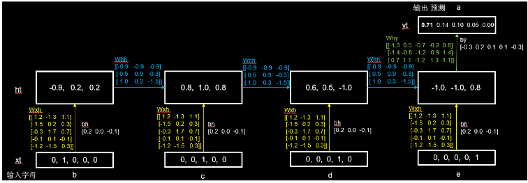
说明有71%的可能是字母a。观察输出结果，模型不仅成功预测出下一个字母a，还可以从神经网络输出的概率发现：因为输入序列的最后一个字母是e，所以模型理应也确实认为下一个字母还是e的可能性最小，可能性最大的是a，其次分别是b、c、d。

（1）4pre1实践

a.用独热编码的方式实现：
 

import numpy as np
import tensorflow as tf
from tensorflow.keras.layers import Dense, SimpleRNN
import matplotlib.pyplot as plt
import os

input_word = "abcde"
w_to_id = {'a': 0, 'b': 1, 'c': 2, 'd': 3, 'e': 4}  # 单词映射到数值id的词典
id_to_onehot = {0: [1., 0., 0., 0., 0.], 1: [0., 1., 0., 0., 0.], 2: [0., 0., 1., 0., 0.], 3: [0., 0., 0., 1., 0.],
                4: [0., 0., 0., 0., 1.]}  # id编码为one-hot

#  与onehot_1pre1不同的地方，即x_train、y_train变成了四个字母预测一个字母的形式（输入连续的abcd对应的标签是e、输入连续的bcde对应的标签是a、依此类推）
x_train = [
    [id_to_onehot[w_to_id['a']], id_to_onehot[w_to_id['b']], id_to_onehot[w_to_id['c']], id_to_onehot[w_to_id['d']]],
    [id_to_onehot[w_to_id['b']], id_to_onehot[w_to_id['c']], id_to_onehot[w_to_id['d']], id_to_onehot[w_to_id['e']]],
    [id_to_onehot[w_to_id['c']], id_to_onehot[w_to_id['d']], id_to_onehot[w_to_id['e']], id_to_onehot[w_to_id['a']]],
    [id_to_onehot[w_to_id['d']], id_to_onehot[w_to_id['e']], id_to_onehot[w_to_id['a']], id_to_onehot[w_to_id['b']]],
    [id_to_onehot[w_to_id['e']], id_to_onehot[w_to_id['a']], id_to_onehot[w_to_id['b']], id_to_onehot[w_to_id['c']]],
]
y_train = [w_to_id['e'], w_to_id['a'], w_to_id['b'], w_to_id['c'], w_to_id['d']]

np.random.seed(7)
np.random.shuffle(x_train)
np.random.seed(7)
np.random.shuffle(y_train)
tf.random.set_seed(7)

# 使x_train符合SimpleRNN输入要求：[送入样本数， 循环核时间展开步数， 每个时间步输入特征个数]。
# 此处整个数据集送入，送入样本数为len(x_train)；输入4个字母出结果，循环核时间展开步数为4; 表示为独热码有5个输入特征，每个时间步输入特征个数为5
x_train = np.reshape(x_train, (len(x_train), 4, 5))
y_train = np.array(y_train)

model = tf.keras.Sequential([
    SimpleRNN(3),
    Dense(5, activation='softmax')
])

model.compile(optimizer=tf.keras.optimizers.Adam(0.01),
              loss=tf.keras.losses.SparseCategoricalCrossentropy(from_logits=False),
              metrics=['sparse_categorical_accuracy'])

checkpoint_save_path = "./checkpoint/rnn_onehot_4pre1.ckpt"

if os.path.exists(checkpoint_save_path + '.index'):
    print('-------------load the model-----------------')
    model.load_weights(checkpoint_save_path)

cp_callback = tf.keras.callbacks.ModelCheckpoint(filepath=checkpoint_save_path,
                                                 save_weights_only=True,
                                                 save_best_only=True,
                                                 monitor='loss')  # 由于fit没有给出测试集，不计算测试集准确率，根据loss，保存最优模型

history = model.fit(x_train, y_train, batch_size=32, epochs=100, callbacks=[cp_callback])

model.summary()

# print(model.trainable_variables)
file = open('./weights.txt', 'w')  # 参数提取
for v in model.trainable_variables:
    file.write(str(v.name) + '\n')
    file.write(str(v.shape) + '\n')
    file.write(str(v.numpy()) + '\n')
file.close()

###############################################    show   ###############################################

# 显示训练集和验证集的acc和loss曲线
acc = history.history['sparse_categorical_accuracy']
loss = history.history['loss']

plt.subplot(1, 2, 1)
plt.plot(acc, label='Training Accuracy')
plt.title('Training Accuracy')
plt.legend()

plt.subplot(1, 2, 2)
plt.plot(loss, label='Training Loss')
plt.title('Training Loss')
plt.legend()
plt.show()

############### predict #############

preNum = int(input("input the number of test alphabet:"))
for i in range(preNum):
    alphabet1 = input("input test alphabet:")
    alphabet = [id_to_onehot[w_to_id[a]] for a in alphabet1]
    # 使alphabet符合SimpleRNN输入要求：[送入样本数， 循环核时间展开步数， 每个时间步输入特征个数]。此处验证效果送入了1个样本，送入样本数为1；输入4个字母出结果，所以循环核时间展开步数为4; 表示为独热码有5个输入特征，每个时间步输入特征个数为5
    alphabet = np.reshape(alphabet, (1, 4, 5))
    result = model.predict([alphabet])
    pred = tf.argmax(result, axis=1)
    pred = int(pred)
    tf.print(alphabet1 + '->' + input_word[pred])

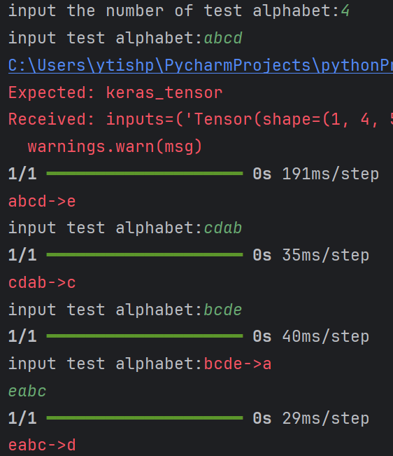
在结果预测时，需要等待连续输入四个字母，然后把这四个字母转换为独热码，然后调整为RNN层希望的形状输入网络进行预测即可。运行结果如下图：

b.用Embedding编码的方式实现：

      这次将词汇量扩充到26个（即字母从a到z），首先建立一个映射表，把字母用数字表示为0到25；然后建立两个空列表，一个用于存放训练用的输入特征x_train，另一个用于存放训练用的标签y_train；接下来用for循环从数字列表中把连续4个数作为输入特征添加到x_train中，第5个数做为标签添加到y_train中，这就构建了训练用的输入特征x_train和标签y_train。

input_word = "abcdefghijklmnopqrstuvwxyz"
w_to_id = {'a': 0, 'b': 1, 'c': 2, 'd': 3, 'e': 4,
           'f': 5, 'g': 6, 'h': 7, 'i': 8, 'j': 9,
           'k': 10, 'l': 11, 'm': 12, 'n': 13, 'o': 14,
           'p': 15, 'q': 16, 'r': 17, 's': 18, 't': 19,
           'u': 20, 'v': 21, 'w': 22, 'x': 23, 'y': 24, 'z': 25}  # 单词映射到数值id的词典

training_set_scaled = [0, 1, 2, 3, 4, 5, 6, 7, 8, 9, 10,
                       11, 12, 13, 14, 15, 16, 17, 18, 19, 20,
                       21, 22, 23, 24, 25]

x_train = []
y_train = []

for i in range(4, 26):
    x_train.append(training_set_scaled[i - 4:i])
    y_train.append(training_set_scaled[i])

        把输入特征变成Embedding层期待的形状才能输入网络；在sequntial搭建网络时，相比于one_hot形式增加了一层Embedding层，先对输入数据进行编码，这里的26表示词汇量是26，这里的2表示每个单词用2个数值编码，这一层会生成一个26行2列的可训练参数矩阵，实现编码可训练。随后设定具有十个记忆体的循环层和一个全连接层（输出会是26个字母之一，所以这里是26）；后边进行compile、fit、summary、参数提取和acc/loss可视化是和前面的代码一样。

# 使x_train符合Embedding输入要求：[送入样本数， 循环核时间展开步数] ，
# 此处整个数据集送入所以送入，送入样本数为len(x_train)；输入4个字母出结果，循环核时间展开步数为4。
x_train = np.reshape(x_train, (len(x_train), 4))
y_train = np.array(y_train)

model = tf.keras.Sequential([
    Embedding(26, 2),
    SimpleRNN(10),
    Dense(26, activation='softmax')
])

在预测环节，与one_hot同样的操作，测试结果如下

preNum = int(input("input the number of test alphabet:"))
for i in range(preNum):
    alphabet1 = input("input test alphabet:")
    alphabet = [w_to_id[a] for a in alphabet1]
    # 使alphabet符合Embedding输入要求：[送入样本数， 时间展开步数]。
    # 此处验证效果送入了1个样本，送入样本数为1；输入4个字母出结果，循环核时间展开步数为4。
    alphabet = np.reshape(alphabet, (1, 4))
    result = model.predict([alphabet])
    pred = tf.argmax(result, axis=1)
    pred = int(pred)
    tf.print(alphabet1 + '->' + input_word[pred])

7、RNN实现股票预测

（1）数据源：SH600519.csv是用tushare模块下载的SH600519贵州茅台的日k线数据，本次列子中只用到C列数据：用连续60天的开盘价，预测第61天的开盘价。

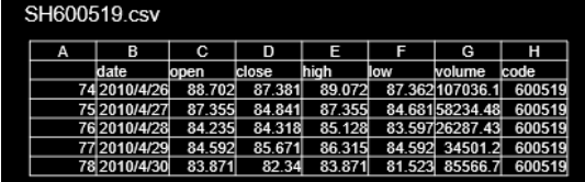
    整个过程按照六步法：import相关模块、读取k线数据到变量maotai，把变量maotai中前2126天数据中的开盘价作为训练数据，把变量maotai中后300天数据中的开盘价作为测试数据；然后对开盘价进行归一化，使送入神经网络的数据分布在0到1之间；接下来建立空列表分别用于接收训练集输入特征、训练集标签、测试集输入特征、测试集标签；

import numpy as np
import tensorflow as tf
from tensorflow.keras.layers import Dropout, Dense, SimpleRNN
import matplotlib.pyplot as plt
import os
import pandas as pd
from sklearn.preprocessing import MinMaxScaler
from sklearn.metrics import mean_squared_error, mean_absolute_error
import math

maotai = pd.read_csv('./SH600519.csv')  # 读取股票文件

training_set = maotai.iloc[0:2426 - 300, 2:3].values  # 前(2426-300=2126)天的开盘价作为训练集,表格从0开始计数，2:3 是提取[2:3)列，前闭后开,故提取出C列开盘价
test_set = maotai.iloc[2426 - 300:, 2:3].values  # 后300天的开盘价作为测试集

# 归一化
sc = MinMaxScaler(feature_range=(0, 1))  # 定义归一化：归一化到(0，1)之间
training_set_scaled = sc.fit_transform(training_set)  # 求得训练集的最大值，最小值这些训练集固有的属性，并在训练集上进行归一化
test_set = sc.transform(test_set)  # 利用训练集的属性对测试集进行归一化

x_train = []
y_train = []

x_test = []
y_test = []

      继续构造数据。用for循环遍历整个训练数据，没连续60天数据作为输入特征x_train，第61天数据作为对应的标签y_train，一共生成2066组训练数据，然后打乱训练数据的顺序并转变为array格式继而转变为RNN输入要求的维度，同理，测试集一样的操作，但是测试集不打乱顺序。

# 测试集：csv表格中前2426-300=2126天数据
# 利用for循环，遍历整个训练集，提取训练集中连续60天的开盘价作为输入特征x_train，第61天的数据作为标签，for循环共构建2426-300-60=2066组数据。
for i in range(60, len(training_set_scaled)):
    x_train.append(training_set_scaled[i - 60:i, 0])
    y_train.append(training_set_scaled[i, 0])
# 对训练集进行打乱
np.random.seed(7)
np.random.shuffle(x_train)
np.random.seed(7)
np.random.shuffle(y_train)
tf.random.set_seed(7)
# 将训练集由list格式变为array格式
x_train, y_train = np.array(x_train), np.array(y_train)

# 使x_train符合RNN输入要求：[送入样本数， 循环核时间展开步数， 每个时间步输入特征个数]。
# 此处整个数据集送入，送入样本数为x_train.shape[0]即2066组数据；输入60个开盘价，预测出第61天的开盘价，循环核时间展开步数为60; 每个时间步送入的特征是某一天的开盘价，只有1个数据，故每个时间步输入特征个数为1
x_train = np.reshape(x_train, (x_train.shape[0], 60, 1))
# 测试集：csv表格中后300天数据
# 利用for循环，遍历整个测试集，提取测试集中连续60天的开盘价作为输入特征x_train，第61天的数据作为标签，for循环共构建300-60=240组数据。
for i in range(60, len(test_set)):
    x_test.append(test_set[i - 60:i, 0])
    y_test.append(test_set[i, 0])
# 测试集变array并reshape为符合RNN输入要求：[送入样本数， 循环核时间展开步数， 每个时间步输入特征个数]
x_test, y_test = np.array(x_test), np.array(y_test)
x_test = np.reshape(x_test, (x_test.shape[0], 60, 1))

       用sequntial搭建神经网络：第一层循环计算层记忆体设定80个，每个时间步推送发给下一层，使用0.2的Dropout；第二层循环计算层设定记忆体有100个，仅最后的时间推送给下一层，使用0.2的Dropout；由于输出值是第61天的开盘价只有一个数，所以全连接Dense是1

model = tf.keras.Sequential([
    SimpleRNN(80, return_sequences=True),
    Dropout(0.2),
    SimpleRNN(100),
    Dropout(0.2),
    Dense(1)
])

      compile配置训练方法使用adam优化器，使用均方误差损失函数。在股票预测代码中，只需要观测loss，训练迭代打印的时候也只打印loss，所以这里就无需给metrics赋值、设置断点训练，fit执行训练过程、summary打印出网络结构和参数统计。

model.compile(optimizer=tf.keras.optimizers.Adam(0.001),
              loss='mean_squared_error')  # 损失函数用均方误差
# 该应用只观测loss数值，不观测准确率，所以删去metrics选项，一会在每个epoch迭代显示时只显示loss值

checkpoint_save_path = "./checkpoint/rnn_stock.ckpt"

if os.path.exists(checkpoint_save_path + '.index'):
    print('-------------load the model-----------------')
    model.load_weights(checkpoint_save_path)

cp_callback = tf.keras.callbacks.ModelCheckpoint(filepath=checkpoint_save_path,
                                                 save_weights_only=True,
                                                 save_best_only=True,
                                                 monitor='val_loss')

history = model.fit(x_train, y_train, batch_size=64, epochs=50, validation_data=(x_test, y_test), validation_freq=1,
                    callbacks=[cp_callback])

model.summary()

file = open('./weights.txt', 'w')  # 参数提取
for v in model.trainable_variables:
    file.write(str(v.name) + '\n')
    file.write(str(v.shape) + '\n')
    file.write(str(v.numpy()) + '\n')
file.close()

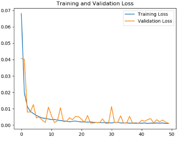
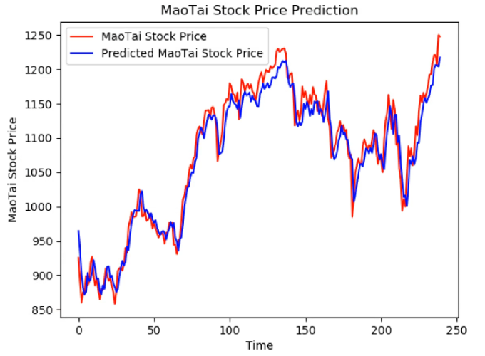
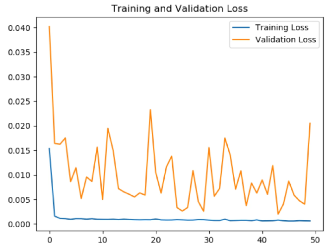
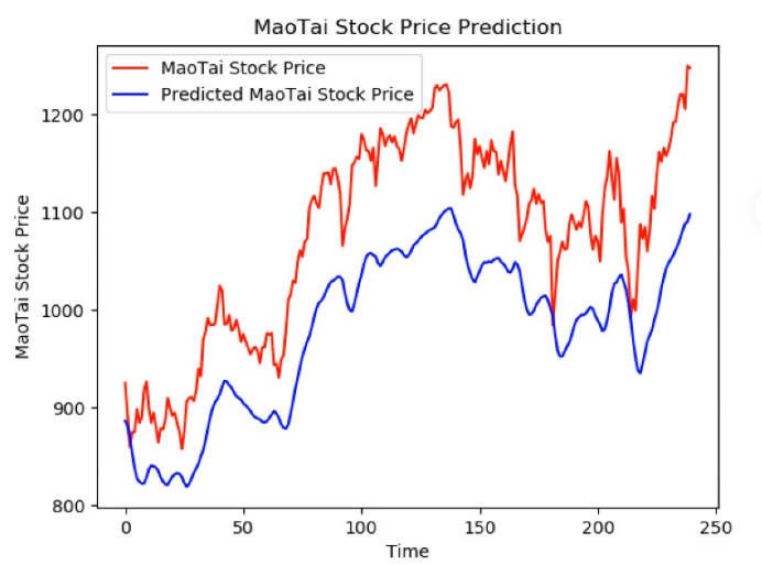
       进行股票的预测。用predict预测测试集数据，然后将预测值和真实值从归一化的数值变换到真实数值，最后用红色画出真实值曲线、用蓝色线画出预测值曲线。

loss = history.history['loss']
val_loss = history.history['val_loss']

plt.plot(loss, label='Training Loss')
plt.plot(val_loss, label='Validation Loss')
plt.title('Training and Validation Loss')
plt.legend()
plt.show()

################## predict ######################
# 测试集输入模型进行预测
predicted_stock_price = model.predict(x_test)
# 对预测数据还原---从（0，1）反归一化到原始范围
predicted_stock_price = sc.inverse_transform(predicted_stock_price)
# 对真实数据还原---从（0，1）反归一化到原始范围
real_stock_price = sc.inverse_transform(test_set[60:])
# 画出真实数据和预测数据的对比曲线
plt.plot(real_stock_price, color='red', label='MaoTai Stock Price')
plt.plot(predicted_stock_price, color='blue', label='Predicted MaoTai Stock Price')
plt.title('MaoTai Stock Price Prediction')
plt.xlabel('Time')
plt.ylabel('MaoTai Stock Price')
plt.legend()
plt.show()

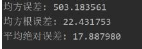
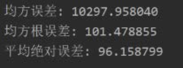
      为评价模型优劣，给出了三个评判指标：均方误差、均方根误差和平均绝对误差，这些误差越小说明预测的数值与真实值越接近。

##########evaluate##############
# calculate MSE 均方误差 ---> E[(预测值-真实值)^2] (预测值减真实值求平方后求均值)
mse = mean_squared_error(predicted_stock_price, real_stock_price)
# calculate RMSE 均方根误差--->sqrt[MSE]    (对均方误差开方)
rmse = math.sqrt(mean_squared_error(predicted_stock_price, real_stock_price))
# calculate MAE 平均绝对误差----->E[|预测值-真实值|](预测值减真实值求绝对值后求均值）
mae = mean_absolute_error(predicted_stock_price, real_stock_price)
print('均方误差: %.6f' % mse)
print('均方根误差: %.6f' % rmse)
print('平均绝对误差: %.6f' % mae)

loss值曲线

股票预测曲线

股票预测评价指标

二、LSTM

1、RNN出现的问题：无法解决长跨度依赖问题，即后面节点相对于跨度很大的前面时间节点的信息感知能力太弱。

eg.在短句子中的词可以由短跨度的词预测出来，而较长跨度的词很难预测出来。

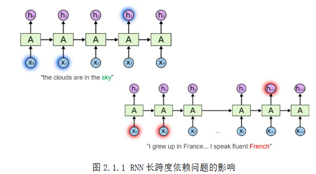
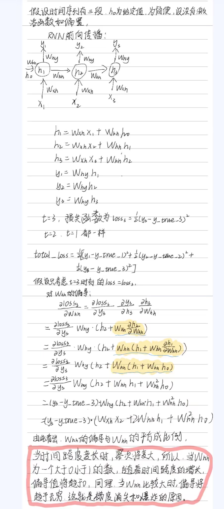
长跨度依赖的根本问题在于，多阶段的反向传播后会导致梯度消失、梯度爆炸。（可以看知乎上韦伟作者的相关作品）可以使用梯度截断去解决梯度爆炸问题，但无法轻易解决梯度消失问题。

下面举例解释RNN梯度消失和爆炸的原因：
 

2、LSTM

LSTM通过门控单元很好的解决了RNN长期依赖问题。

（1）原理：为解决长期依赖问题，LSTM采用了门（gate）机制对信息的流通和损失进行了控制。

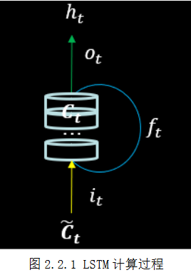
采用了三个门限：输入门、遗忘门、输出门；引入了表征长期记忆的细胞态，引入了等待存入长期记忆的候选态：

（2）三个门限都是当前时刻的输入特征和上个时刻的短期记忆的函数，分别表示为：

输入门（门限）：，决定了多少比例的信息会被存入当前细胞态；

遗忘门（门限）：，将细胞态中的信息选择性的遗忘；

输出门（门限）：，将细胞态中的信息选择性的进行输出；

三个公式中、和是待训练参数矩阵，、和是待训练偏置项。为sigmoid激活函数，它可以使门限的范围在0到1之间。

（3）定义为记忆体，它表征短期记忆，是当前细胞态经过输出们得到的：记忆体（短期记忆）：

（4）候选态表示归纳出的待存入细胞态的新知识，是当前时刻的输入特征和上一个时刻的短期记忆的函数：

候选态（归纳出的新知识）：

（5）细胞态表示长期记忆，它等于上个时刻的长期记忆通过遗忘门的值和当前时刻归纳出的新知识通过输入门的值之和：

细胞态（长期记忆）：

     假设LSTM就是我们听老师讲课的过程,目前老师讲到了第45页PPT。我们 的脑袋里记住的内容,是PPT第1页到第45页的长期记忆。它由两部分组成: 一部分是PPT第1页到第44页的内容，也就是上一时刻的长期记忆。我们不可能一字不差的记住全部内容，会不自觉地忘记了一些,所以上个时刻的长期记忆要乘以遗忘门,这个乘积项就表示留存在我们脑中的对过去的记忆；另一部分是当前我们归纳出的新知识，它由老师正在讲的第45页PPT(当前时刻的输入)和第44页PPT的短期记忆留存(上一时刻的短期记忆)组成。 将现在的记忆乘以输入门后与过去的记忆一同存储为当前的长期记忆。接下 来,如果我们想把我们学到的知识(当前的长期记忆)复述给朋友,我们不可能 一字不落的讲出来,所以需要经过输出门筛选后才成为了输出。

     当有多层循环网络时,第二层循环网络的输入就是第一层循环网络的输出 ,即输入第二层网络的是第一层网络提取出的精华。可以这么想,老师现在扮演的就是第一层循环网络,每一页PPT都是老师从一篇一篇论文中提取出的精华,输出给我们。作为第二层循环网络的我们,接收到的数据就是老师的长期记忆过 tanh激活函数后乘以输出门提取出的短期记忆ht。

（7）Tensorflow2描述LSTM层

tf.keras.layers.LSTM(神经元个数，return_sequences=是否返回输出)

神经元个数和return_sequences的含义与SimpleRNN相同。

eg.LSTM(8，return_sequences=True)

（8）LSTM股票预测

将RNN预测股票中的模型部分更换为以下代码

model = tf.keras.Sequential([
    LSTM(80, return_sequences=True),
    Dropout(0.2),
    LSTM(100),
    Dropout(0.2),
    Dense(1)
])

运行结果