深入解析分布式训练架构的技术细节。这不是简单的"多卡训练"，而是一个涉及通信拓扑、并行策略、内存管理和调度优化的复杂系统。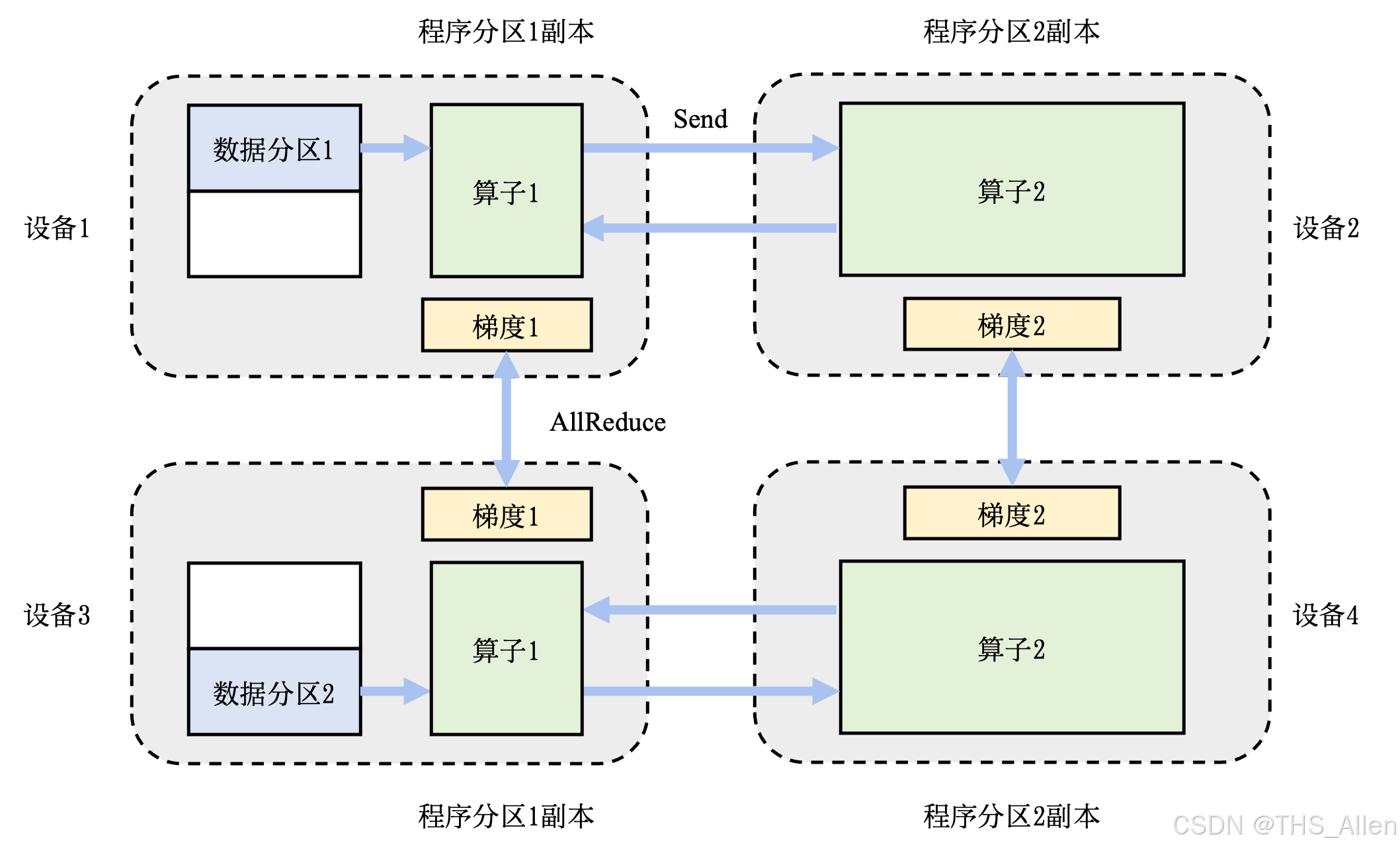

---

一、分布式训练核心挑战与架构演进

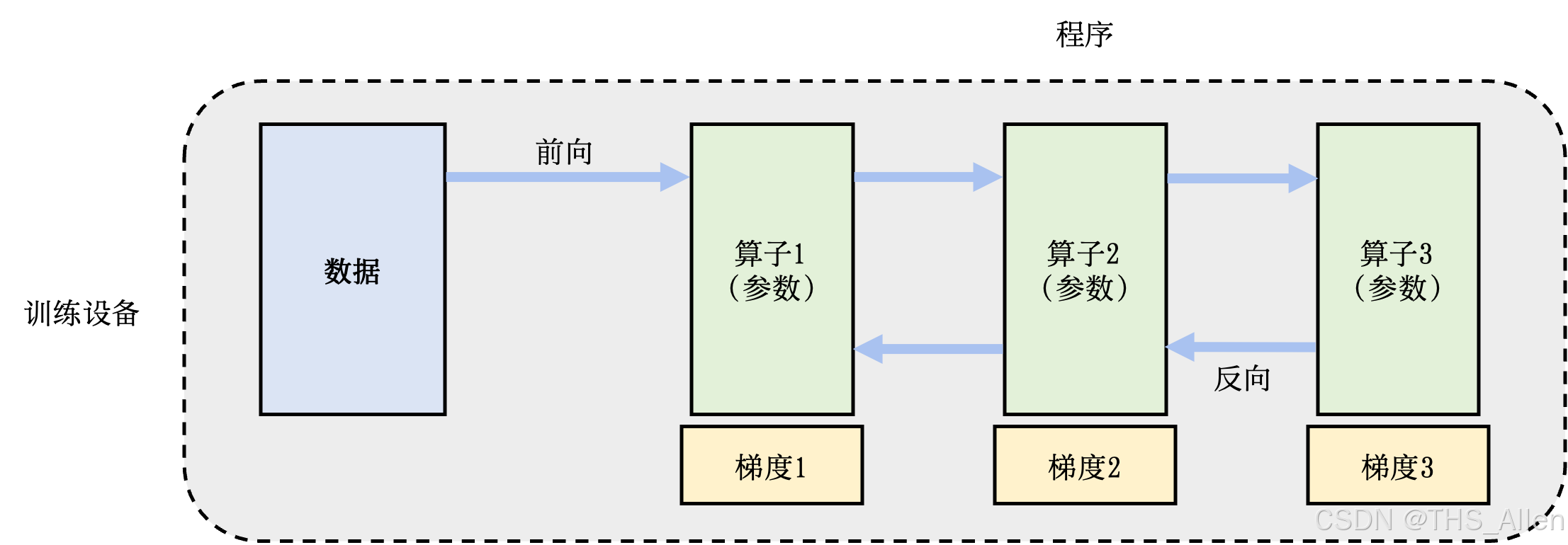
1.1 根本问题：单机极限

# 单机训练的资源瓶颈
class SingleNodeLimits:
    def __init__(self):
        self.gpu_memory = 80 * GB  # A100/H100
        self.pcie_bandwidth = 64 * GB/s  # PCIe 4.0 x16
        self.model_size_limit = 200 * GB  # 实际约100B参数模型
        self.training_time = "weeks to months"

1.2 分布式训练演进路径

单机单卡 → 单机多卡 → 多机多卡 → 超大规模集群

---

二、核心并行策略深度解析

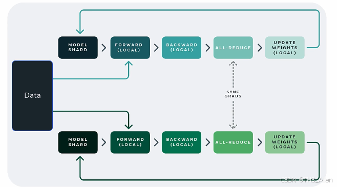
2.1 数据并行：最基础的分布式模式

2.1.1 基础架构

class DataParallelBasics:
    def __init__(self, model, world_size):
        self.model = model
        self.world_size = world_size
        
    def training_step(self, batch):
        # 1. 数据分片
        local_batch = self.split_batch(batch, self.world_size)
        
        # 2. 每个GPU上前向传播
        local_output = self.model(local_batch)
        
        # 3. 计算本地梯度
        local_loss = self.criterion(local_output)
        local_loss.backward()
        
        # 4. 梯度全局同步 (关键步骤!)
        self.average_gradients()
        
        # 5. 参数更新
        self.optimizer.step()

2.1.2 梯度同步算法对比

// 方案1: Parameter Server (传统但低效)
// 工作节点 → 参数服务器 → 工作节点
void parameter_server_sync() {
    // 所有worker发送梯度到PS
    for (int i = 0; i < num_workers; i++) {
        send_gradients_to_ps(worker_grads[i]);
    }
    
    // PS聚合梯度
    averaged_grads = average_all_gradients();
    
    // PS广播聚合后的梯度
    for (int i = 0; i < num_workers; i++) {
        broadcast_gradients_to_worker(averaged_grads, i);
    }
}

// 方案2: All-Reduce (现代高效方案)
void all_reduce_sync() {
    // 使用Ring-AllReduce或Tree-AllReduce
    // 所有节点平等参与，无单点瓶颈
    ring_allreduce(local_gradients, global_gradients, world_size);
}

2.1.3 All-Reduce算法详解

Ring-AllReduce 实现原理：

class RingAllReduce:
    def __init__(self, rank, world_size):
        self.rank = rank
        self.world_size = world_size
        self.left_neighbor = (rank - 1) % world_size
        self.right_neighbor = (rank + 1) % world_size
        
    def all_reduce(self, tensor):
        # 阶段1: Scatter-Reduce
        chunk_size = tensor.numel() // self.world_size
        for step in range(self.world_size - 1):
            send_chunk_idx = (self.rank - step) % self.world_size
            recv_chunk_idx = (self.rank - step - 1) % self.world_size
            
            # 发送当前块，接收邻居块
            send_chunk = tensor[chunk_size*send_chunk_idx: 
                               chunk_size*(send_chunk_idx+1)]
            recv_chunk = torch.empty_like(send_chunk)
            
            # 非阻塞通信
            isend(send_chunk, self.right_neighbor)
            irecv(recv_chunk, self.left_neighbor)
            wait_all()
            
            # 累加接收到的块
            tensor[chunk_size*recv_chunk_idx: 
                  chunk_size*(recv_chunk_idx+1)] += recv_chunk
        
        # 阶段2: All-Gather  
        for step in range(self.world_size - 1):
            send_chunk_idx = (self.rank - step + 1) % self.world_size
            recv_chunk_idx = (self.rank - step) % self.world_size
            
            send_chunk = tensor[chunk_size*send_chunk_idx:
                               chunk_size*(send_chunk_idx+1)]
            recv_chunk = torch.empty_like(send_chunk)
            
            isend(send_chunk, self.right_neighbor)
            irecv(recv_chunk, self.left_neighbor)
            wait_all()
            
            tensor[chunk_size*recv_chunk_idx:
                  chunk_size*(recv_chunk_idx+1)] = recv_chunk

2.2 模型并行：突破单卡内存限制

2.2.1 张量并行（Tensor Parallelism）

class TensorParallelLinear:
    def __init__(self, in_features, out_features, device_mesh):
        self.device_mesh = device_mesh
        self.rank = device_mesh.get_rank()
        
        # 按列拆分权重矩阵
        self.shard_size = out_features // device_mesh.size()
        self.local_weight = nn.Parameter(
            torch.randn(in_features, self.shard_size, 
                       device=device_mesh.device))
        
    def forward(self, x):
        # 本地计算部分结果
        local_output = torch.matmul(x, self.local_weight)  # [B, S, shard_size]
        
        # 在所有设备间收集完整结果
        global_output = all_gather(local_output, self.device_mesh)
        
        # 拼接得到完整输出 [B, S, out_features]
        return torch.cat(global_output, dim=-1)

2.2.2 Transformer层的张量并行实现

class TensorParallelTransformerLayer:
    def __init__(self, hidden_size, num_heads, device_mesh):
        self.device_mesh = device_mesh
        
        # MLP层拆分
        self.mlp_parallel = TensorParallelMLP(hidden_size, device_mesh)
        
        # 注意力层拆分  
        self.attention_parallel = TensorParallelAttention(
            hidden_size, num_heads, device_mesh)
            
    def forward(self, hidden_states):
        # 注意力并行计算
        attention_output = self.attention_parallel(hidden_states)
        
        # MLP并行计算
        mlp_output = self.mlp_parallel(attention_output)
        
        return mlp_output

2.2.3 流水线并行（Pipeline Parallelism）

class PipelineParallelModel:
    def __init__(self, layers, devices):
        self.devices = devices
        self.num_stages = len(devices)
        
        # 将模型层分配到不同设备
        self.stages = []
        layers_per_stage = len(layers) // self.num_stages
        
        for i in range(self.num_stages):
            start_idx = i * layers_per_stage
            end_idx = start_idx + layers_per_stage
            stage_layers = layers[start_idx:end_idx]
            self.stages.append(nn.Sequential(*stage_layers).to(devices[i]))
    
    def forward(self, x, micro_batches=4):
        # 将输入拆分为微批次
        micro_batch_size = x.size(0) // micro_batches
        micro_batches = torch.chunk(x, micro_batches, dim=0)
        
        # 流水线执行
        activations = [None] * (micro_batches + 1)
        activations[0] = [None] * len(micro_batches)
        
        for stage_idx in range(self.num_stages):
            current_device = self.devices[stage_idx]
            
            for mb_idx in range(micro_batches):
                # 将输入移动到当前设备
                if stage_idx == 0:
                    input_mb = micro_batches[mb_idx].to(current_device)
                else:
                    input_mb = activations[stage_idx-1][mb_idx].to(current_device)
                
                # 在当前阶段计算
                with torch.cuda.device(current_device):
                    output_mb = self.stages[stage_idx](input_mb)
                
                activations[stage_idx][mb_idx] = output_mb
        
        # 收集最终输出
        return torch.cat(activations[self.num_stages-1], dim=0)

2.3 3D混合并行：现代大模型训练标准

class Hybrid3DParallel:
    def __init__(self, model_config, parallel_config):
        self.data_parallel_size = parallel_config['dp']
        self.tensor_parallel_size = parallel_config['tp'] 
        self.pipeline_parallel_size = parallel_config['pp']
        
        # 计算总设备数
        self.world_size = dp_size * tp_size * pp_size
        
    def setup_parallelism(self, model):
        # 1. 流水线并行：按层拆分到不同设备组
        pipeline_groups = self.create_pipeline_groups()
        
        # 2. 张量并行：在每个流水线阶段内按张量维度拆分
        tensor_groups = self.create_tensor_groups()
        
        # 3. 数据并行：复制完整的流水线-张量并行单元
        data_parallel_groups = self.create_data_parallel_groups()
        
        return HybridParallelModel(model, {
            'pipeline': pipeline_groups,
            'tensor': tensor_groups, 
            'data': data_parallel_groups
        })

---

三、通信拓扑与硬件感知优化

3.1 硬件拓扑感知的设备放置

class TopologyAwarePlacement:
    def __init__(self, cluster_info):
        self.num_nodes = cluster_info['num_nodes']
        self.gpus_per_node = cluster_info['gpus_per_node']
        self.inter_node_bandwidth = cluster_info['inter_node_bw']
        self.intra_node_bandwidth = cluster_info['intra_node_bw']
    
    def optimize_device_mesh(self, parallel_config):
        # 基于通信模式优化设备网格
        
        # 张量并行：需要高带宽，优先放在节点内
        # 数据并行：可以跨节点，对带宽要求较低
        # 流水线并行：阶段间通信量中等
        
        device_mesh = []
        for pp_rank in range(parallel_config['pp']):
            pp_group = []
            for dp_rank in range(parallel_config['dp']):
                # 为每个数据并行组创建张量并行组
                tp_group = self.get_intra_node_group(parallel_config['tp'])
                pp_group.append(tp_group)
            device_mesh.append(pp_group)
        
        return device_mesh

3.2 通信优化技术

3.2.1 通信计算重叠

class CommunicationOverlap:
    def __init__(self, model, gradient_buffers):
        self.model = model
        self.gradient_buffers = gradient_buffers
        
    def backward_with_overlap(self, loss):
        loss.backward(retain_graph=True)
        
        # 在计算梯度的同时开始通信
        for param in self.model.parameters():
            if param.grad is not None:
                # 非阻塞通信
                handle = dist.all_reduce(
                    param.grad, 
                    op=dist.ReduceOp.AVG, 
                    async_op=True
                )
                self.communication_handles.append(handle)
        
        # 继续下一层的反向传播
        # 通信在后台进行

3.2.2 梯度分桶与压缩

class GradientBucketing:
    def __init__(self, bucket_size_mb=25):
        self.bucket_size = bucket_size_mb * 1024 * 1024  # 25MB
        
    def create_gradient_buckets(self, parameters):
        buckets = []
        current_bucket = []
        current_size = 0
        
        for param in sorted(parameters, key=lambda x: x.numel()):
            param_size = param.numel() * param.element_size()
            
            if current_size + param_size > self.bucket_size and current_bucket:
                buckets.append(current_bucket)
                current_bucket = []
                current_size = 0
            
            current_bucket.append(param)
            current_size += param_size
        
        if current_bucket:
            buckets.append(current_bucket)
            
        return buckets

class GradientCompression:
    def compress_gradients(self, gradients, compression_ratio=0.01):
        # 1. 梯度裁剪和稀疏化
        flattened_grad = torch.cat([g.view(-1) for g in gradients])
        
        # 2. 选择top-k梯度
        k = int(flattened_grad.numel() * compression_ratio)
        values, indices = torch.topk(flattened_grad.abs(), k)
        
        # 3. 只通信重要的梯度
        sparse_grad = (values, indices)
        return sparse_grad

---

四、现代分布式训练框架实现

4.1 基于PyTorch Distributed的实现

import torch.distributed as dist
from torch.nn.parallel import DistributedDataParallel as DDP

class ModernDistributedTrainer:
    def __init__(self, model, train_loader, config):
        self.setup_distributed_environment(config)
        self.model = self.wrap_model(model)
        self.optimizer = self.create_optimizer()
        
    def setup_distributed_environment(self, config):
        # 初始化进程组
        dist.init_process_group(
            backend='nccl',
            init_method='env://',
            world_size=config['world_size'],
            rank=config['rank']
        )
        
        # 设置设备
        local_rank = config['local_rank']
        torch.cuda.set_device(local_rank)
        
    def wrap_model(self, model):
        # 使用DDP包装模型
        model = model.cuda()
        model = DDP(
            model,
            device_ids=[self.local_rank],
            output_device=self.local_rank,
            find_unused_parameters=True,
            gradient_as_bucket_view=True  # 内存优化
        )
        return model
    
    def training_epoch(self):
        self.model.train()
        
        for batch in self.train_loader:
            # 将数据移动到当前设备
            batch = self.move_to_device(batch)
            
            # 前向传播
            outputs = self.model(batch)
            loss = self.criterion(outputs)
            
            # 反向传播 (DDP自动处理梯度同步)
            self.optimizer.zero_grad()
            loss.backward()
            
            # 梯度裁剪
            torch.nn.utils.clip_grad_norm_(
                self.model.parameters(), 
                max_norm=1.0
            )
            
            # 参数更新
            self.optimizer.step()
            
            # 可选的: 学习率调度
            self.scheduler.step()

4.2 Megatron-LM风格的高级并行

class MegatronStyleParallel:
    def __init__(self, model_config, parallel_config):
        self.tensor_parallel_size = parallel_config['tp']
        self.pipeline_parallel_size = parallel_config['pp']
        
    def create_parallel_transformer(self):
        # 列并行线性层
        self.attention_dense = ColumnParallelLinear(
            hidden_size, 
            hidden_size * 3,  # Q, K, V
            gather_output=False
        )
        
        # 行并行线性层  
        self.output_dense = RowParallelLinear(
            hidden_size,
            hidden_size,
            input_is_parallel=True
        )
        
    def tensor_parallel_attention(self, hidden_states):
        # 拆分QKV计算
        mixed_x = self.attention_dense(hidden_states)  # [s, b, 3h]
        
        # 在张量并行组内拆分头
        new_x_shape = mixed_x.size()[:-1] + (
            self.num_heads, 3 * self.hidden_size_per_head)
        mixed_x = mixed_x.view(*new_x_shape)  # [s, b, n, 3h]
        
        # 在最后一个维度拆分Q, K, V
        last_dim = mixed_x.size(-1)
        last_dim = last_dim // self.tensor_parallel_size
        
        # 本地只处理部分头
        local_mixed_x = mixed_x[...,
            self.rank*last_dim:(self.rank+1)*last_dim]
        
        # 本地注意力计算
        local_q, local_k, local_v = torch.split(
            local_mixed_x, self.hidden_size_per_head, dim=-1)
        
        # ... 本地注意力计算
        return local_attention_output

---

五、弹性训练与容错机制

5.1 动态节点调度

class ElasticTrainingManager:
    def __init__(self, checkpoint_dir, min_nodes, max_nodes):
        self.checkpoint_dir = checkpoint_dir
        self.min_nodes = min_nodes
        self.max_nodes = max_nodes
        
    def monitor_cluster_health(self):
        while True:
            current_nodes = self.get_available_nodes()
            
            # 节点数量变化处理
            if len(current_nodes) != self.current_world_size:
                self.handle_scale_event(current_nodes)
            
            time.sleep(60)  # 每分钟检查一次
    
    def handle_scale_event(self, new_nodes):
        # 1. 保存检查点
        self.save_checkpoint()
        
        # 2. 重新配置并行策略
        new_parallel_config = self.recompute_parallel_config(new_nodes)
        
        # 3. 重新初始化进程组
        dist.destroy_process_group()
        self.setup_distributed_environment(new_parallel_config)
        
        # 4. 从检查点恢复
        self.load_checkpoint()

5.2 检查点与恢复

class CheckpointManager:
    def save_checkpoint(self, model, optimizer, step):
        # 分布式保存检查点
        if self.rank == 0:
            # 主节点保存模型和优化器状态
            checkpoint = {
                'model_state_dict': model.state_dict(),
                'optimizer_state_dict': optimizer.state_dict(),
                'step': step,
                'world_size': self.world_size
            }
            torch.save(checkpoint, f'checkpoint_{step}.pt')
        
        # 所有节点等待保存完成
        dist.barrier()
    
    def load_checkpoint(self, checkpoint_path):
        # 加载检查点并处理可能的世界大小变化
        checkpoint = torch.load(checkpoint_path, map_location='cpu')
        
        # 处理模型状态字典的形状不匹配
        if checkpoint['world_size'] != self.world_size:
            self.reshape_state_dict_for_new_world_size(
                checkpoint['model_state_dict']
            )
        
        model.load_state_dict(checkpoint['model_state_dict'])
        optimizer.load_state_dict(checkpoint['optimizer_state_dict'])
        
        return checkpoint['step']

---

六、性能监控与调优

6.1 分布式训练指标收集

class DistributedMetrics:
    def __init__(self):
        self.communication_time = 0
        self.computation_time = 0
        self.idle_time = 0
        
    def profile_training_step(self):
        # 记录各阶段时间
        comp_start = time.time()
        # ... 前向传播和反向传播计算
        comp_end = time.time()
        
        comm_start = time.time()
        # ... 梯度同步
        comm_end = time.time()
        
        self.computation_time += (comp_end - comp_start)
        self.communication_time += (comm_end - comm_start)
        
    def calculate_efficiency(self):
        total_time = self.computation_time + self.communication_time
        computation_efficiency = self.computation_time / total_time
        
        # 理想情况下，计算效率应 > 80%
        return computation_efficiency

6.2 自动并行策略搜索

class ParallelStrategySearcher:
    def search_optimal_strategy(self, model_size, cluster_info):
        strategies = self.generate_candidate_strategies(
            model_size, cluster_info)
        
        best_strategy = None
        best_throughput = 0
        
        for strategy in strategies:
            estimated_throughput = self.estimate_throughput(
                strategy, cluster_info)
            
            if estimated_throughput > best_throughput:
                best_throughput = estimated_throughput
                best_strategy = strategy
        
        return best_strategy
    
    def estimate_throughput(self, strategy, cluster_info):
        # 基于通信计算比的吞吐量估计
        computation_time = self.estimate_computation_time(strategy)
        communication_time = self.estimate_communication_time(
            strategy, cluster_info)
        
        # 考虑通信计算重叠
        effective_time = max(computation_time, communication_time)
        
        return strategy.micro_batch_size / effective_time

---

总结

现代分布式训练架构是一个多层次、多维度的复杂系统，其核心要点包括：

1. 并行策略组合：数据并行、模型并行、流水线并行的有机结合
2. 通信优化：All-Reduce算法、通信计算重叠、梯度压缩等技术
3. 硬件感知：基于实际硬件拓扑的设备放置和通信优化
4. 弹性容错：支持动态扩缩容和故障恢复
5. 性能调优：基于监控数据的自动策略优化

成功的分布式训练系统需要在算法效率、硬件利用率和工程复杂度之间找到最佳平衡。随着模型规模的持续增长，分布式训练架构将继续向更细粒度、更自适应、更智能的方向演进。