深度学习与神经网络之分类问题
也就是说自变量和因变量之间存在线性关系,实际问题中我们会遇到很多数据之间并非是线性关系,因此我们引入新的概念广义线性回归。分类问题:垃圾邮件识别,图片分类,疾病判断分类器:能够自动对输入的数据进行分类输入:特征,输出:离散值实现分类器:1.准备训练样本2.训练分类器3.对新样本进行分类交叉熵损失函数。
1.1 逻辑回归
线性回归:
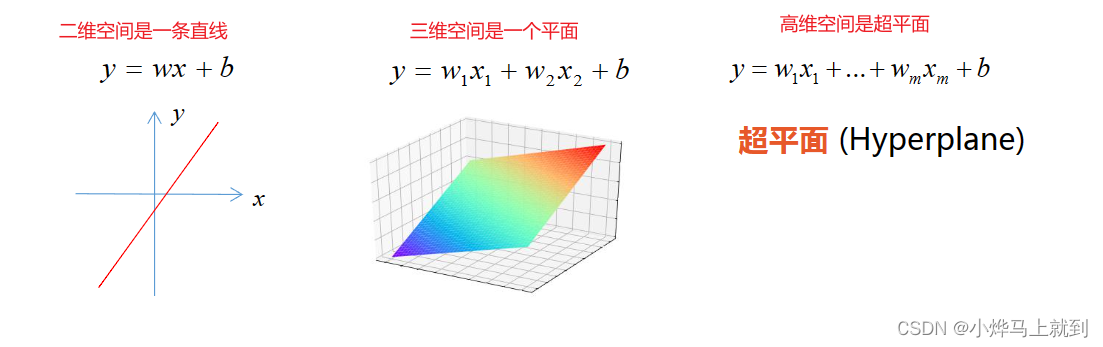
线性回归就是将自变量和因变量之间的关系,用线性模型表示,也就是说自变量和因变量之间存在线性关系,使我们能够根据已知的样本数据,对未来或者未知的数据进行估计。
实际问题中我们会遇到很多数据之间并非是线性关系,因此我们引入新的概念广义线性回归。

分类问题:垃圾邮件识别,图片分类,疾病判断
分类器:能够自动对输入的数据进行分类
输入:特征,输出:离散值

实现分类器:
1.准备训练样本
2.训练分类器
3.对新样本进行分类


交叉熵损失函数


1.2 实现一元逻辑回归-Tensorflow

sigmoid()函数
import tensorflow as tf
import numpy as np

# sigmoid
x = np.array([1., 2., 3., 4.])
w = tf.Variable(1.)
b = tf.Variable(1.)

y = 1 / (1 + tf.exp(- (w * x + b)))
交叉熵损失函数
import tensorflow as tf
import numpy as np
# 交叉熵损失函数
y = np.array([0, 0, 1, 1])
pred = np.array([0.1, 0.2, 0.8, 0.49])
Loss = -tf.reduce_sum(y * tf.math.log(pred) + (1 - y) * tf.math.log(1 - pred))
# 平均交叉熵损失函数
avgLoss = -tf.reduce_mean(y * tf.math.log(pred) + (1 - y) * tf.math.log(1 - pred))
准确率
import tensorflow as tf
import numpy as np

y = np.array([0, 0 ,1 ,1])
pred = np.array([0.1, 0.2, 0.8, 0.49])

tf.round(pred)
tf.equal(tf.round(pred), y)
accuracy = tf.reduce_mean(tf.cast(tf.equal(tf.round(pred), y), tf.float32))
1.3 房屋销售记录demo
1.准备数据

2.加载数据
import tensorflow as tf
import numpy as np
import matplotlib.pyplot as plt

x = np.array([137.97, 104.50, 100.00, 126.32, 79.20, 99.00, 124.00, 114.00,
                 106.69, 140.05, 53.75, 46.91, 68.00, 63.02, 81.26, 86.21])
y = np.array([1, 1, 0, 1, 0, 1, 1, 0, 0, 1, 0, 0, 0, 0, 0, 0])

plt.scatter(x, y)
plt.show()
3.数据处理,由于sigmoid函数是以零点为中心的,因此对数据进行中心化处理
import tensorflow as tf
import numpy as np
import matplotlib.pyplot as plt

# 加载数据
x = np.array([137.97, 104.50, 100.00, 126.32, 79.20, 99.00, 124.00, 114.00,
                 106.69, 140.05, 53.75, 46.91, 68.00, 63.02, 81.26, 86.21])
y = np.array([1, 1, 0, 1, 0, 1, 1, 0, 0, 1, 0, 0, 0, 0, 0, 0])

# 数据处理
x_train = x - np.mean(x)
y_train = y

plt.scatter(x_train, y_train)
plt.show()
数据相对位置没变,但是被整体平移。

4.设置超参数和模型变量初始值
# 设置超参数
learn_rate = 0.005
iter = 5

display_step = 1

# 设置模型变量初始值
np.random.seed(612)
w = tf.Variable(np.random.randn())
b = tf.Variable(np.random.randn())
5.训练模型
import tensorflow as tf
import numpy as np
import matplotlib.pyplot as plt

# 加载数据
x = np.array([137.97, 104.50, 100.00, 126.32, 79.20, 99.00, 124.00, 114.00,
                 106.69, 140.05, 53.75, 46.91, 68.00, 63.02, 81.26, 86.21])
y = np.array([1, 1, 0, 1, 0, 1, 1, 0, 0, 1, 0, 0, 0, 0, 0, 0])

# 数据处理
x_train = x - np.mean(x)
y_train = y

# 设置超参数
learn_rate = 0.005
iter = 5

display_step = 1

# 设置模型变量初始值
np.random.seed(612)
w = tf.Variable(np.random.randn())
b = tf.Variable(np.random.randn())

# 训练模型
cross_train = []  # 存放训练集的交叉熵损失
acc_train = []     # 用来存放训练集的分类准确率

for i in range(0, iter + 1):
    with tf.GradientTape() as type:
        pred_train = 1 / (1 + tf.exp(- (w * x_train + b)))
        Loss_train = - tf.reduce_mean(y_train * tf.math.log(pred_train) + (1 - y_train) * tf.math.log(1 - pred_train))
        Accuracy_train = tf.reduce_mean(tf.cast(tf.equal(tf.where(pred_train < 0.5, 0, 1), y_train), tf.float32))

    cross_train.append(Loss_train)
    acc_train.append(Accuracy_train)
    dL_dw, dL_db = type.gradient(Loss_train, [w,b])

    w.assign_sub(learn_rate * dL_dw)
    b.assign_sub(learn_rate * dL_db)

    if i % display_step == 0:
        print("i: %i, Train Loss: %f, Accuracy: %f" %(i, Loss_train, Accuracy_train))

6.使用初始权值的sigmoid函数
# 使用初始权值的sigmoid函数
np.random.seed(612)
w = tf.Variable(np.random.randn())
b = tf.Variable(np.random.randn())
x_ = range(-80, 80)
y_ = 1 / (1+ tf.exp(- (w * x_ +b)))
plt.plot(x_, y_)
plt.show()

7.绘制所有的sigmoid函数曲线
import tensorflow as tf
import numpy as np
import matplotlib.pyplot as plt

# 加载数据
x = np.array([137.97, 104.50, 100.00, 126.32, 79.20, 99.00, 124.00, 114.00,
                 106.69, 140.05, 53.75, 46.91, 68.00, 63.02, 81.26, 86.21])
y = np.array([1, 1, 0, 1, 0, 1, 1, 0, 0, 1, 0, 0, 0, 0, 0, 0])

# 数据处理
x_train = x - np.mean(x)
y_train = y

# 设置超参数
learn_rate = 0.005
iter = 5

display_step = 1

# 设置模型变量初始值
np.random.seed(612)
w = tf.Variable(np.random.randn())
b = tf.Variable(np.random.randn())
x_ = range(-80, 80)
y_ = 1 / (1+ tf.exp(- (w * x_ +b)))

# 训练模型
plt.scatter(x_train, y_train)
plt.plot(x_, y_, color ="red", linewidth=3)
cross_train = []  # 存放训练集的交叉熵损失
acc_train = []     # 用来存放训练集的分类准确率

for i in range(0, iter + 1):
    with tf.GradientTape() as type:
        pred_train = 1 / (1 + tf.exp(- (w * x_train + b)))
        Loss_train = - tf.reduce_mean(y_train * tf.math.log(pred_train) + (1 - y_train) * tf.math.log(1 - pred_train))
        Accuracy_train = tf.reduce_mean(tf.cast(tf.equal(tf.where(pred_train < 0.5, 0, 1), y_train), tf.float32))

    cross_train.append(Loss_train)
    acc_train.append(Accuracy_train)
    dL_dw, dL_db = type.gradient(Loss_train, [w,b])

    w.assign_sub(learn_rate * dL_dw)
    b.assign_sub(learn_rate * dL_db)

    if i % display_step == 0:
        print("i: %i, Train Loss: %f, Accuracy: %f" %(i, Loss_train, Accuracy_train))
        y_ = 1 / (1 + tf.exp(- (w * x_ + b)))
        plt.plot(x_, y_)

plt.show()

8.对训练好的模型进行商品房分类和结果可视化
import tensorflow as tf
import numpy as np
import matplotlib.pyplot as plt

# 加载数据
x = np.array([137.97, 104.50, 100.00, 126.32, 79.20, 99.00, 124.00, 114.00,
                 106.69, 140.05, 53.75, 46.91, 68.00, 63.02, 81.26, 86.21])
y = np.array([1, 1, 0, 1, 0, 1, 1, 0, 0, 1, 0, 0, 0, 0, 0, 0])

# 数据处理
x_train = x - np.mean(x)
y_train = y

# 设置超参数
learn_rate = 0.005
iter = 5

display_step = 1

# 设置模型变量初始值
np.random.seed(612)
w = tf.Variable(np.random.randn())
b = tf.Variable(np.random.randn())
x_ = range(-80, 80)
y_ = 1 / (1+ tf.exp(- (w * x_ +b)))

# 训练模型
cross_train = []  # 存放训练集的交叉熵损失
acc_train = []     # 用来存放训练集的分类准确率

for i in range(0, iter + 1):
    with tf.GradientTape() as type:
        pred_train = 1 / (1 + tf.exp(- (w * x_train + b)))
        Loss_train = - tf.reduce_mean(y_train * tf.math.log(pred_train) + (1 - y_train) * tf.math.log(1 - pred_train))
        Accuracy_train = tf.reduce_mean(tf.cast(tf.equal(tf.where(pred_train < 0.5, 0, 1), y_train), tf.float32))

    cross_train.append(Loss_train)
    acc_train.append(Accuracy_train)
    dL_dw, dL_db = type.gradient(Loss_train, [w,b])

    w.assign_sub(learn_rate * dL_dw)
    b.assign_sub(learn_rate * dL_db)

    if i % display_step == 0:
        print("i: %i, Train Loss: %f, Accuracy: %f" %(i, Loss_train, Accuracy_train))


x_test = [128.15, 45.00, 141.43, 106.27, 99.00, 53.84, 85.36, 70.00, 162.00, 114.60]
pred_test = 1 / (1 + tf.exp(- (w * (x_test - np.mean(x)) + b)))
y_test = tf.where(pred_test < 0.5, 0, 1)
for i in range(len(x_test)):
    print(x_test[i], "\t\t", pred_test[i].numpy(), "\t\t", y_test[i].numpy(), "\t\t")

plt.scatter(x_test, y_test)
x_ = np.array(range(-80, 80))
y_ = 1 / (1 + tf.exp(- (w * x_ +b)))
plt.plot(x_ + np.mean(x), y_)
plt.show()
1.4 线性分类器 (决策边界)
一维空间:将两个数据集分开的点
二维空间:将两个数据集分开的线
二维空间:将两个数据集分开的面


非线性可分:无法通过一条直线划分

逻辑运算

1.5 多元逻辑回归
鸢尾花数据集特征:
- 150个样本
- 4个属性
- 花萼长度
- 花萼宽度
- 花瓣长度
- 花瓣宽度
- 一个标签
- 山鸢尾
- 变色鸢尾
- 维吉尼亚鸢尾
通过花萼长度和花萼宽度逻辑回归实现山鸢尾和变色鸢尾的分类
import tensorflow.keras as keras
import pandas as pd
import numpy as np
import matplotlib.pyplot as plt
import matplotlib as mpl
import tensorflow as tf

TRAIN_URL = "https://download.tensorflow.org/data/iris_training.csv"
train_path = keras.utils.get_file(TRAIN_URL.split("/")[-1], TRAIN_URL)

df_iris = pd.read_csv(train_path, header=0)

# 处理数据
""""
1.转化为NumPy数组
2.提取属性和标签
3.提取山鸢尾和变色鸢尾
"""
iris = np.array(df_iris)
train_x = iris[:, 0:2]
train_y = iris[:, 4]
x_train = train_x[train_y < 2]
y_train = train_y[train_y < 2]
num = len(x_train)
# 属性中心化
x_train = x_train - np.mean(x_train, axis=0)
# 生成多元模型的属性矩阵和标签列向量
x0_train = np.ones(num).reshape(-1, 1)
X = tf.cast(tf.concat((x0_train, x_train), axis=1), tf.float32)
Y = tf.cast(y_train.reshape(-1, 1), tf.float32)

# 设置超参数
learn_rate = 0.2
iter = 120
display_step = 30
# 设置模型参数初始值
np.random.seed(612)
W = tf.Variable(np.random.randn(3, 1), dtype=tf.float32)

# 训练模型
cm_pt = mpl.colors.ListedColormap(["blue", "red"])
plt.scatter(x_train[:, 0], x_train[:, 1], c=y_train, cmap=cm_pt)
x_ = [-1.5, 1.5]
y_ = -(W[1] * x_ + W[0]) / W[2]
plt.plot(x_, y_, color="red", linewidth=3)
plt.xlim([-1.5, 1.5])
plt.ylim([-1.5, 1.5])
ce = []
acc = []
for i in range(0, iter + 1):
    with tf.GradientTape() as tape:
        PRED = 1 / (1 + tf.exp(- tf.matmul(X, W)))
        Loss = -tf.reduce_mean(Y * tf.math.log(PRED) + (1 - Y) * tf.math.log(1 - PRED))

    accuracy = tf.reduce_mean(tf.cast(tf.equal(tf.where(PRED.numpy() < 0.5, 0., 1.), Y), tf.float32))
    ce.append(Loss)
    acc.append(accuracy)
    dL_dW = tape.gradient(Loss, W)
    W.assign_sub(learn_rate * dL_dW)

    if i % display_step == 0:
        print("i: %i, Acc: %f, Loss: %f" % (i, accuracy, Loss))
        y_ = - (W[0] + W[1] * x_) / W[2]
        plt.plot(x_, y_)


plt.show()
使用测试集来评价模型的性能
import tensorflow.keras as keras
import pandas as pd
import numpy as np
import matplotlib.pyplot as plt
import matplotlib as mpl
import tensorflow as tf

TRAIN_URL = "http://download.tensorflow.org/data/iris_training.csv"
train_path = keras.utils.get_file(TRAIN_URL.split("/")[-1], TRAIN_URL)
TEST_URL = "http://download.tensorflow.org/data/iris_test.csv"
test_path = keras.utils.get_file(TEST_URL.split("/")[-1], TEST_URL)

df_iris_train = pd.read_csv(train_path, header=0)
df_iris_test = pd.read_csv(test_path, header=0)

# 处理数据
""""
1.转化为NumPy数组
2.提取属性和标签
3.提取山鸢尾和变色鸢尾
"""
iris_train = np.array(df_iris_train)
iris_test = np.array(df_iris_test)
train_x = iris_train[:, 0:2]
train_y = iris_train[:, 4]
test_x = iris_test[:, 0:2]
test_y = iris_test[:, 4]
x_train = train_x[train_y < 2]
y_train = train_y[train_y < 2]
x_test = test_x[test_y < 2]
y_test = test_y[test_y < 2]
num_train = len(x_train)
num_test = len(x_test)

# 属性中心化
x_train = x_train - np.mean(x_train, axis=0)
x_test = x_test - np.mean(x_test, axis=0)
# 生成多元模型的属性矩阵和标签列向量
x0_train = np.ones(num_train).reshape(-1, 1)
X_train = tf.cast(tf.concat((x0_train, x_train), axis=1), tf.float32)
Y_train = tf.cast(y_train.reshape(-1, 1), dtype=tf.float32)
x0_test = np.ones(num_test).reshape(-1, 1)
X_test = tf.cast(tf.concat((x0_test, x_test), axis=1), tf.float32)
Y_test = tf.cast(y_test.reshape(-1, 1), dtype=tf.float32)

# 设置超参数
learn_rate = 0.2
iter = 120
display_step = 30
# 设置模型参数初始值
np.random.seed(612)
W = tf.Variable(np.random.randn(3, 1), dtype=tf.float32)

# 训练模型
ce_train = []
acc_train = []
ce_test = []
acc_test = []
for i in range(0, iter + 1):
    with tf.GradientTape() as tape:
        PRED_train = 1 / (1 + tf.exp(- tf.matmul(X_train, W)))
        Loss_train = -tf.reduce_mean(Y_train * tf.math.log(PRED_train) + (1 - Y_train) * tf.math.log(1 - PRED_train))
        PRED_test = 1 / (1 + tf.exp(- tf.matmul(X_test, W)))
        Loss_test = -tf.reduce_mean(Y_test * tf.math.log(PRED_test) + (1 - Y_test) * tf.math.log(1 - PRED_test))

    accuracy_train = tf.reduce_mean(tf.cast(tf.equal(tf.where(PRED_train.numpy() < 0.5, 0., 1.), Y_train), tf.float32))
    accuracy_test = tf.reduce_mean(tf.cast(tf.equal(tf.where(PRED_test.numpy() < 0.5, 0., 1.), Y_test), tf.float32))

    ce_train.append(Loss_train)
    acc_train.append(accuracy_train)
    ce_test.append(Loss_test)
    acc_test.append(accuracy_test)

    dL_dW = tape.gradient(Loss_train, W)
    W.assign_sub(learn_rate * dL_dW)

    if i % display_step == 0:
        print("i: %i, Acc_train: %f, Loss_train: %f, Acc_test: %f, Loss_test: %f" % (
        i, accuracy_train, Loss_train, accuracy_test, Loss_test))


# 可视化训练集和测试集的损失函数和准确率
plt.figure(figsize=(10, 3))

plt.subplot(121)
plt.plot(ce_train, color="blue", label="train")
plt.plot(ce_test, color="red", label="test")
plt.ylabel("Loss")
plt.legend()

plt.subplot(122)
plt.plot(acc_train, color="blue", label="train")
plt.plot(acc_test, color="red", label="test")
plt.ylabel("Accuracy")

plt.legend()
plt.show()

1.6 绘制分类图
生成网格坐标矩阵np.meshgrid() 填充网格plt.pcolomesh()
import tensorflow as tf
import numpy as np
import matplotlib.pyplot as plt
import matplotlib as mpl

n = 10 # n值越大,颜色过度越细腻
x = np.linspace(-10, 10, n)
y = np.linspace(-10, 10, n)
X, Y = np.meshgrid(x, y)
Z = X + Y
plt.pcolormesh(X, Y, Z, cmap="rainbow")
plt.show()
训练集根据鸢尾花分类模型绘制分类图
import tensorflow.keras as keras
import pandas as pd
import numpy as np
import matplotlib.pyplot as plt
import matplotlib as mpl
import tensorflow as tf

TRAIN_URL = "http://download.tensorflow.org/data/iris_training.csv"
train_path = keras.utils.get_file(TRAIN_URL.split("/")[-1], TRAIN_URL)
TEST_URL = "http://download.tensorflow.org/data/iris_test.csv"
test_path = keras.utils.get_file(TEST_URL.split("/")[-1], TEST_URL)

df_iris_train = pd.read_csv(train_path, header=0)
df_iris_test = pd.read_csv(test_path, header=0)

# 处理数据
""""
1.转化为NumPy数组
2.提取属性和标签
3.提取山鸢尾和变色鸢尾
"""
iris_train = np.array(df_iris_train)
iris_test = np.array(df_iris_test)
train_x = iris_train[:, 0:2]
train_y = iris_train[:, 4]
test_x = iris_test[:, 0:2]
test_y = iris_test[:, 4]
x_train = train_x[train_y < 2]
y_train = train_y[train_y < 2]
x_test = test_x[test_y < 2]
y_test = test_y[test_y < 2]
num_train = len(x_train)
num_test = len(x_test)

# 属性中心化
x_train = x_train - np.mean(x_train, axis=0)
x_test = x_test - np.mean(x_test, axis=0)
# 生成多元模型的属性矩阵和标签列向量
x0_train = np.ones(num_train).reshape(-1, 1)
X_train = tf.cast(tf.concat((x0_train, x_train), axis=1), tf.float32)
Y_train = tf.cast(y_train.reshape(-1, 1), dtype=tf.float32)
x0_test = np.ones(num_test).reshape(-1, 1)
X_test = tf.cast(tf.concat((x0_test, x_test), axis=1), tf.float32)
Y_test = tf.cast(y_test.reshape(-1, 1), dtype=tf.float32)

# 设置超参数
learn_rate = 0.2
iter = 120
display_step = 30
# 设置模型参数初始值
np.random.seed(612)
W = tf.Variable(np.random.randn(3, 1), dtype=tf.float32)

# 训练模型
ce_train = []
acc_train = []
ce_test = []
acc_test = []
for i in range(0, iter + 1):
    with tf.GradientTape() as tape:
        PRED_train = 1 / (1 + tf.exp(- tf.matmul(X_train, W)))
        Loss_train = -tf.reduce_mean(Y_train * tf.math.log(PRED_train) + (1 - Y_train) * tf.math.log(1 - PRED_train))
        PRED_test = 1 / (1 + tf.exp(- tf.matmul(X_test, W)))
        Loss_test = -tf.reduce_mean(Y_test * tf.math.log(PRED_test) + (1 - Y_test) * tf.math.log(1 - PRED_test))

    accuracy_train = tf.reduce_mean(tf.cast(tf.equal(tf.where(PRED_train.numpy() < 0.5, 0., 1.), Y_train), tf.float32))
    accuracy_test = tf.reduce_mean(tf.cast(tf.equal(tf.where(PRED_test.numpy() < 0.5, 0., 1.), Y_test), tf.float32))

    ce_train.append(Loss_train)
    acc_train.append(accuracy_train)
    ce_test.append(Loss_test)
    acc_test.append(accuracy_test)

    dL_dW = tape.gradient(Loss_train, W)
    W.assign_sub(learn_rate * dL_dW)

    if i % display_step == 0:
        print("i: %i, Acc_train: %f, Loss_train: %f, Acc_test: %f, Loss_test: %f" % (
        i, accuracy_train, Loss_train, accuracy_test, Loss_test))


# 训练集根据鸢尾花分类模型绘制分类图
M = 300
x1_min, x2_min = x_train.min(axis=0)
x1_max, x2_max = x_train.max(axis=0)
t1 = np.linspace(x1_min, x1_max, M)
t2 = np.linspace(x2_min, x2_max, M)
m1, m2 = np.meshgrid(t1, t2)

m0 = np.ones(M * M)
X_mesh = tf.cast(np.stack((m0, m1.reshape(-1), m2.reshape(-1)),axis=1),dtype=tf.float32)
Y_mesh = tf.cast(1 / (1 + tf.exp(-tf.matmul(X_mesh, W))),dtype=tf.float32)
Y_mesh = tf.where(Y_mesh < 0.5, 0, 1)
n = tf.reshape(Y_mesh, m1.shape)

cm_pt = mpl.colors.ListedColormap(["blue", "red"])
cm_bg = mpl.colors.ListedColormap(["#FD971F", "#A6E22E"])
plt.pcolormesh(m1, m2, n, cmap=cm_bg, shading='auto')  # 添加shading='auto'以改善外观
plt.scatter(x_train[:, 0], x_train[:, 1], c=y_train, cmap=cm_pt)
plt.show()

测试集根据鸢尾花分类模型绘制分类图
import tensorflow.keras as keras
import pandas as pd
import numpy as np
import matplotlib.pyplot as plt
import matplotlib as mpl
import tensorflow as tf

TRAIN_URL = "http://download.tensorflow.org/data/iris_training.csv"
train_path = keras.utils.get_file(TRAIN_URL.split("/")[-1], TRAIN_URL)
TEST_URL = "http://download.tensorflow.org/data/iris_test.csv"
test_path = keras.utils.get_file(TEST_URL.split("/")[-1], TEST_URL)

df_iris_train = pd.read_csv(train_path, header=0)
df_iris_test = pd.read_csv(test_path, header=0)

# 处理数据
""""
1.转化为NumPy数组
2.提取属性和标签
3.提取山鸢尾和变色鸢尾
"""
iris_train = np.array(df_iris_train)
iris_test = np.array(df_iris_test)
train_x = iris_train[:, 0:2]
train_y = iris_train[:, 4]
test_x = iris_test[:, 0:2]
test_y = iris_test[:, 4]
x_train = train_x[train_y < 2]
y_train = train_y[train_y < 2]
x_test = test_x[test_y < 2]
y_test = test_y[test_y < 2]
num_train = len(x_train)
num_test = len(x_test)

# 属性中心化
x_train = x_train - np.mean(x_train, axis=0)
x_test = x_test - np.mean(x_test, axis=0)
# 生成多元模型的属性矩阵和标签列向量
x0_train = np.ones(num_train).reshape(-1, 1)
X_train = tf.cast(tf.concat((x0_train, x_train), axis=1), tf.float32)
Y_train = tf.cast(y_train.reshape(-1, 1), dtype=tf.float32)
x0_test = np.ones(num_test).reshape(-1, 1)
X_test = tf.cast(tf.concat((x0_test, x_test), axis=1), tf.float32)
Y_test = tf.cast(y_test.reshape(-1, 1), dtype=tf.float32)

# 设置超参数
learn_rate = 0.2
iter = 120
display_step = 30
# 设置模型参数初始值
np.random.seed(612)
W = tf.Variable(np.random.randn(3, 1), dtype=tf.float32)

# 训练模型
ce_train = []
acc_train = []
ce_test = []
acc_test = []
for i in range(0, iter + 1):
    with tf.GradientTape() as tape:
        PRED_train = 1 / (1 + tf.exp(- tf.matmul(X_train, W)))
        Loss_train = -tf.reduce_mean(Y_train * tf.math.log(PRED_train) + (1 - Y_train) * tf.math.log(1 - PRED_train))
        PRED_test = 1 / (1 + tf.exp(- tf.matmul(X_test, W)))
        Loss_test = -tf.reduce_mean(Y_test * tf.math.log(PRED_test) + (1 - Y_test) * tf.math.log(1 - PRED_test))

    accuracy_train = tf.reduce_mean(tf.cast(tf.equal(tf.where(PRED_train.numpy() < 0.5, 0., 1.), Y_train), tf.float32))
    accuracy_test = tf.reduce_mean(tf.cast(tf.equal(tf.where(PRED_test.numpy() < 0.5, 0., 1.), Y_test), tf.float32))

    ce_train.append(Loss_train)
    acc_train.append(accuracy_train)
    ce_test.append(Loss_test)
    acc_test.append(accuracy_test)

    dL_dW = tape.gradient(Loss_train, W)
    W.assign_sub(learn_rate * dL_dW)

    if i % display_step == 0:
        print("i: %i, Acc_train: %f, Loss_train: %f, Acc_test: %f, Loss_test: %f" % (
        i, accuracy_train, Loss_train, accuracy_test, Loss_test))


# 测试集根据鸢尾花分类模型绘制分类图
M = 300
x1_min, x2_min = x_test.min(axis=0)
x1_max, x2_max = x_test.max(axis=0)
t1 = np.linspace(x1_min, x1_max, M)
t2 = np.linspace(x2_min, x2_max, M)
m1, m2 = np.meshgrid(t1, t2)

m0 = np.ones(M * M)
X_mesh = tf.cast(np.stack((m0, m1.reshape(-1), m2.reshape(-1)),axis=1),dtype=tf.float32)
Y_mesh = tf.cast(1 / (1 + tf.exp(-tf.matmul(X_mesh, W))),dtype=tf.float32)
Y_mesh = tf.where(Y_mesh < 0.5, 0, 1)
n = tf.reshape(Y_mesh, m1.shape)

cm_pt = mpl.colors.ListedColormap(["blue", "red"])
cm_bg = mpl.colors.ListedColormap(["#FD971F", "#A6E22E"])
plt.pcolormesh(m1, m2, n, cmap=cm_bg, shading='auto')  # 添加shading='auto'以改善外观
plt.scatter(x_test[:, 0], x_test[:, 1], c=y_test, cmap=cm_pt)
plt.show()

1.7 多分类问题


1.8 实现多分类问题
使用花瓣长度、花瓣宽度将三种鸢尾花区分开
import tensorflow.keras as keras
import pandas as pd
import numpy as np
import matplotlib.pyplot as plt
import matplotlib as mpl
import tensorflow as tf

TRAIN_URL = "http://download.tensorflow.org/data/iris_training.csv"
train_path = keras.utils.get_file(TRAIN_URL.split("/")[-1], TRAIN_URL)

df_iris_train = pd.read_csv(train_path, header=0)

# 处理数据
iris_train = np.array(df_iris_train)
x_train = iris_train[:, 2:4]
y_train = iris_train[:, 4]
num_train = len(x_train)

x0_train = np.ones(num_train).reshape(-1, 1)
X_train = tf.cast(tf.concat([x0_train, x_train], axis=1), tf.float32)
# 将鸢尾花标签值转换为独热编码
Y_train = tf.one_hot(tf.constant(y_train, dtype=tf.int32), 3)

# 设置超参数,设置模型参数初始值
learn_rate = 0.2
iter = 500
display_step = 100

np.random.seed(612)
W = tf.Variable(np.random.randn(3, 3), dtype=tf.float32)

# 训练模型
acc = []  # 准确率
cce = []  # 交叉熵损失

for i in range(0, iter + 1):
    with tf.GradientTape() as tape:

        PRED_train = tf.nn.softmax(tf.matmul(X_train, W))  # 计算预测值
        Loss_train = -tf.reduce_sum(Y_train * tf.math.log(PRED_train)) / num_train

    accuracy = tf.reduce_mean(tf.cast(tf.equal(tf.argmax(PRED_train, axis=1), y_train), tf.float32))

    acc.append(accuracy)
    cce.append(Loss_train)
    # 更新模型参数
    dL_dW = tape.gradient(Loss_train, W)
    W.assign_sub(learn_rate * dL_dW)

    if i % display_step == 0:
        print("i: %i, Acc: %f, Loss: %f" % (i, accuracy, Loss_train))

# 训练结果并转化为自然顺序码
tf.reduce_sum(PRED_train, axis=1)
tf.argmax(PRED_train, axis=1)

# 绘制分类图
M = 500
x1_min, x2_min = x_train.min(axis=0)
x1_max, x2_max = x_train.max(axis=0)
t1 = np.linspace(x1_min, x1_max, M)
t2 = np.linspace(x2_min, x2_max, M)
m1, m2 = np.meshgrid(t1, t2)

m0 = np.ones(M * M)
X_ = tf.cast(np.stack((m0, m1.reshape(-1), m2.reshape(-1)),axis=1), tf.float32)
Y_ = tf.nn.softmax(tf.matmul(X_, W))
Y_ = tf.argmax(Y_, axis=1)
n = tf.reshape(Y_, m1.shape)

# 可视化
plt.figure(figsize=(8, 6))

cm_bg = mpl.colors.ListedColormap(["#A0FFA0","#FFA0A0","#A0A0FF"])
plt.pcolormesh(m1, m2, n, cmap=cm_bg)
plt.scatter(x_train[:, 0], x_train[:, 1], c=y_train, cmap="brg")

plt.show()

腾讯云面向开发者汇聚海量精品云计算使用和开发经验,营造开放的云计算技术生态圈。
更多推荐


 7
7 0
0- 0


 已为社区贡献1条内容

所有评论(0)