Yolov 8源码超详细逐行解读+ 网络结构细讲(自我用的小白笔记)
以上就是今天要讲的内容,本文仅仅简单介绍了源码结构,后面还会持续更新讲解,由于这次写的太多了,怕大家看不过来。过段时间继续拆封代码并尝试用常见的pytorch原始框架复现缩减版yolov8。也许上面还有很多错误,欢迎大家指正!!!t=N658t=N658完整且详细的Yolov8复现+训练自己的数据集_咕哥的博客-CSDN博客https://blog.csdn.net/chenhaogu/artic
YOLO V8网络结构
由于作者之前的Yolov8 复现受到了部分好评,所以决定继续从小白学习路线,进行复现代码,磕代码,学理论知识。
代码复现:
完整且详细的Yolov8复现+训练自己的数据集_咕哥的博客-CSDN博客 https://blog.csdn.net/chenhaogu/article/details/131161374?spm=1001.2014.3001.5501(若觉得简单易上手,创作不易,请点赞收藏,谢谢大家!)
提示:若只想关注代码讲解,直接从代码讲解部分看即可。作者初衷为“拆封装,看本质,换自己”,在了解核心代码后,用自己的方式重写没有封装的网络结构。
一、主体网络结构
1、Backbone:主体是CSPDarkNet结构。
yolov5和yolov8主体都是该结构,yolov5主要体现思想的结构是c3模块;yolov8主要体现思想的是c2f模块。
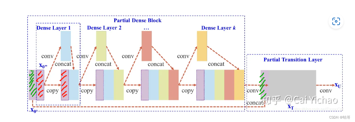
2、CSPnet(Cross Stage Partial):
想要更细致了解的可看知乎一位博主的介绍,非常详细。
CSPNet——PyTorch实现CSPDenseNet和CSPResNeXt - 知乎 (zhihu.com)https://zhuanlan.zhihu.com/p/263555330
总体来说是参考了DenesNet,减少了计算量和增强梯度(不了解DenesNet的同学可以再csdn或者知乎都可以搜到相关论文,若想节省时间简略了解,可加上讲解等字眼。)。可描述为一部分进入卷积网络进行计算,一部分保留最后concat。而在中间过程也有restnet的思想。用一句名言总结莫过于:大肠包小肠。
3、Partial Transition Layer:
对比这四种结构,发现各有其优点。图a是传统的密集型网络思想。图b是图c和图d的综合考虑。图c是part1和part2的大量特征信息最终得以使用,图d这是对一部分进行利用,计算量得以缩小。

4、代码讲解:
(1)网络结构:

(2)网络模型文件保存在models->v8->yolov8.yaml
# YOLOv8.0n backbone
backbone:
# [from, repeats, module, args]
- [-1, 1, Conv, [64, 3, 2]] # 0-P1/2
- [-1, 1, Conv, [128, 3, 2]] # 1-P2/4
- [-1, 3, C2f, [128, True]]
- [-1, 1, Conv, [256, 3, 2]] # 3-P3/8
- [-1, 6, C2f, [256, True]]
- [-1, 1, Conv, [512, 3, 2]] # 5-P4/16
- [-1, 6, C2f, [512, True]]
- [-1, 1, Conv, [1024, 3, 2]] # 7-P5/32
- [-1, 3, C2f, [1024, True]]
- [-1, 1, SPPF, [1024, 5]] # 9
from:输入。-1表示上层的输出作为本层的输入。
repeats:模块的重复次数。
module:使用的模块。
args:模块里面的参数
计算size的公式:out_size =( in_size - k +2 * p)/ s + 1
(3)卷积的代码(nn->modules->conv.py)
def autopad(k, p=None, d=1): # kernel, padding, dilation
"""Pad to 'same' shape outputs."""
if d > 1:
k = d * (k - 1) + 1 if isinstance(k, int) else [d * (x - 1) + 1 for x in k] # actual kernel-size
if p is None:
p = k // 2 if isinstance(k, int) else [x // 2 for x in k] # auto-pad
return p
class Conv(nn.Module):
"""Standard convolution with args(ch_in, ch_out, kernel, stride, padding, groups, dilation, activation)."""
default_act = nn.SiLU() # default activation
def __init__(self, c1, c2, k=1, s=1, p=None, g=1, d=1, act=True):
"""Initialize Conv layer with given arguments including activation."""
super().__init__()
self.conv = nn.Conv2d(c1, c2, k, s, autopad(k, p, d), groups=g, dilation=d, bias=False)
self.bn = nn.BatchNorm2d(c2)
self.act = self.default_act if act is True else act if isinstance(act, nn.Module) else nn.Identity()
def forward(self, x):
"""Apply convolution, batch normalization and activation to input tensor."""
return self.act(self.bn(self.conv(x)))
def forward_fuse(self, x):
"""Perform transposed convolution of 2D data."""
return self.act(self.conv(x))
conv(x)-> bn() -> SiLU()
imput map channel:3 size:640*640
第0层(Conv[3,2,1]) channel:64 size:320*320
第1层(Conv[3,2,1]) channel:128 size:160*160
(4)开始进入核心模块c2f,代码在(nn->modules->block.py)
class C2f(nn.Module):
"""CSP Bottleneck with 2 convolutions."""
def __init__(self, c1, c2, n=1, shortcut=False, g=1, e=0.5): # ch_in, ch_out, number, shortcut, groups, expansion
super().__init__()
self.c = int(c2 * e) # hidden channels
self.cv1 = Conv(c1, 2 * self.c, 1, 1)
self.cv2 = Conv((2 + n) * self.c, c2, 1) # optional act=FReLU(c2)
self.m = nn.ModuleList(Bottleneck(self.c, self.c, shortcut, g, k=((3, 3), (3, 3)), e=1.0) for _ in range(n))
def forward(self, x):
"""Forward pass through C2f layer."""
y = list(self.cv1(x).chunk(2, 1))
y.extend(m(y[-1]) for m in self.m)
return self.cv2(torch.cat(y, 1))
def forward_split(self, x):
"""Forward pass using split() instead of chunk()."""
y = list(self.cv1(x).split((self.c, self.c), 1))
y.extend(m(y[-1]) for m in self.m)
return self.cv2(torch.cat(y, 1))
[-1, 3, C2f, [128, True]]: 3:重复3次C2f; True:Bottleneck有shortcut
难懂代码在于:
self.m = nn.ModuleList(Bottleneck(self.c, self.c, shortcut, g, k=((3, 3), (3, 3)), e=1.0) for _ in range(n))
n:表示n个bottleneck,假设3个,rang(3) -> m:[Bottleneck,Bottleneck;Bottleneck],m此时相当于一个集成的模块。
可以看到三个通道参数,c1=输入通道数;c2=输出通道数;c=0.5*输出通道数;下面是假设输入为[2,128,160,160]各个块的参数。

x先经过cv1 ;
接着开始不同维度的分块,torch.chunk(块数,维度),这里chunk(2,1)是第一维度分成两块;
m(y[-1]) for m in self.m:意思是把第二块放进n个Bottleneck里,等价于:
##举例对比
m(y[-1]) for m in self.m x*x for x in range(3)
=>
for m in self.m: for x in range(3):
m(y[-1]) print(x*x)
##流程,假设3个Bottleneck
Bottleneck0->m m(y[-1]);y.extend加上去 0 -> x -> 0*0=0
Bottleneck1->m m(y[-1]);y.extend加上去 1 -> x -> 1*1=1
Bottleneck2->m m(y[-1]);y.extend加上去 2 -> x -> 2*2=4
y=[Bottleneck0处理过的第二部分,
Bottleneck1处理过的第二部分,
Bottleneck2处理过的第二部分]
因此,y变成2+n块;
torch.cat(y, 1) 将y的第一维度拼接在一起(因为上面chnk是在第一维度分割);
最后经过cv2, featuremap.size 128*160*160。
imput map channel:3 size:640*640
第0层(Conv[3,2,1]) channel:64 size:320*320
第1层(Conv[3,2,1]) channel:128 size:160*160
第2层(C2f)* 3 channel:128 size:160*160
经过一层Conv
imput map channel:3 size:640*640
第0层(Conv[3,2,1]) channel:64 size:320*320
第1层(Conv[3,2,1]) channel:128 size:160*160
第2层(C2f)* 3 channel:128 size:160*160
第3层(Conv[3,2,1]) channel:256 size: 80*80
经过6*C2f,这一层后开始进入常见金字塔型结构连接检测头,检测头部份后面再细讲
C2F部分讲解和上面一致,这次是6个重复模块。
imput map channel:3 size:640*640
第0层(Conv[3,2,1]) channel:64 size:320*320
第1层(Conv[3,2,1]) channel:128 size:160*160
第2层(C2f)* 3 channel:128 size:160*160
第3层(Conv[3,2,1]) channel:256 size: 80*80
第4层(C2f)* 6 channel:256 size: 80*80
经过一层Conv
imput map channel:3 size:640*640
第0层(Conv[3,2,1]) channel:64 size:320*320
第1层(Conv[3,2,1]) channel:128 size:160*160
第2层(C2f)* 3 channel:128 size:160*160
第3层(Conv[3,2,1]) channel:256 size: 80*80
第4层(C2f)* 6 channel:256 size: 80*80
第5层(Conv[3,2,1]) channel:512 size: 40*40
经过6*C2f
imput map channel:3 size:640*640
第0层(Conv[3,2,1]) channel:64 size:320*320
第1层(Conv[3,2,1]) channel:128 size:160*160
第2层(C2f)* 3 channel:128 size:160*160
第3层(Conv[3,2,1]) channel:256 size: 80*80
第4层(C2f)* 6 channel:256 size: 80*80
第5层(Conv[3,2,1]) channel:512 size: 40*40
第6层(C2f)* 6 channel:512 size: 40*40
经过一层Conv
imput map channel:3 size:640*640
第0层(Conv[3,2,1]) channel:64 size:320*320
第1层(Conv[3,2,1]) channel:128 size:160*160
第2层(C2f)* 3 channel:128 size:160*160
第3层(Conv[3,2,1]) channel:256 size: 80*80
第4层(C2f)* 6 channel:256 size: 80*80
第5层(Conv[3,2,1]) channel:512 size: 40*40
第6层(C2f)* 6 channel:512 size: 40*40
第7层(Conv[3,2,1]) channel:512 size: 20*20
经过3*C2f
imput map channel:3 size:640*640
第0层(Conv[3,2,1]) channel:64 size:320*320
第1层(Conv[3,2,1]) channel:128 size:160*160
第2层(C2f)* 3 channel:128 size:160*160
第3层(Conv[3,2,1]) channel:256 size: 80*80
第4层(C2f)* 6 channel:256 size: 80*80
第5层(Conv[3,2,1]) channel:512 size: 40*40
第6层(C2f)* 6 channel:512 size: 40*40
第7层(Conv[3,2,1]) channel:512 size: 20*20
第8层(C2f)* 3 channel:512 size: 20*20
(6)SPPF,代码在(nn->modules->block.py)
imput map channel:3 size:640*640
第0层(Conv[3,2,1]) channel:64 size:320*320
第1层(Conv[3,2,1]) channel:128 size:160*160
第2层(C2f)* 3 channel:128 size:160*160
第3层(Conv[3,2,1]) channel:256 size: 80*80
第4层(C2f)* 6 channel:256 size: 80*80
第5层(Conv[3,2,1]) channel:512 size: 40*40
第6层(C2f)* 6 channel:512 size: 40*40
第7层(Conv[3,2,1]) channel:1024 size: 20*20
第8层(C2f)* 3 channel:1024 size: 20*20
第9层(SPPF[k=5]) channel:1024 size: 20*20

代码:
class SPPF(nn.Module):
"""Spatial Pyramid Pooling - Fast (SPPF) layer for YOLOv5 by Glenn Jocher."""
def __init__(self, c1, c2, k=5): # equivalent to SPP(k=(5, 9, 13))
super().__init__()
c_ = c1 // 2 # hidden channels
self.cv1 = Conv(c1, c_, 1, 1)
self.cv2 = Conv(c_ * 4, c2, 1, 1)
self.m = nn.MaxPool2d(kernel_size=k, stride=1, padding=k // 2)
def forward(self, x):
"""Forward pass through Ghost Convolution block."""
x = self.cv1(x)
y1 = self.m(x)
y2 = self.m(y1)
return self.cv2(torch.cat((x, y1, y2, self.m(y2)), 1))
maxpool的计算公式:

二、Head
1、已经讲解完backbone,下面讲解一下检测头部分
代码如下:(代码在ultralytics -> models -> v8 ->yolov8.yaml)
# YOLOv8.0n head
head:
- [-1, 1, nn.Upsample, [None, 2, 'nearest']]
- [[-1, 6], 1, Concat, [1]] # cat backbone P4
- [-1, 3, C2f, [512]] # 12
- [-1, 1, nn.Upsample, [None, 2, 'nearest']]
- [[-1, 4], 1, Concat, [1]] # cat backbone P3
- [-1, 3, C2f, [256]] # 15 (P3/8-small)
- [-1, 1, Conv, [256, 3, 2]]
- [[-1, 12], 1, Concat, [1]] # cat head P4
- [-1, 3, C2f, [512]] # 18 (P4/16-medium)
- [-1, 1, Conv, [512, 3, 2]]
- [[-1, 9], 1, Concat, [1]] # cat head P5
- [-1, 3, C2f, [1024]] # 21 (P5/32-large)
- [[15, 18, 21], 1, Detect, [nc]] # Detect(P3, P4, P5)
(1)第10层:经过SSPF的模块,接着进入上采样upsample。
None:不指定输出尺寸。
2:输出的尺寸为输入尺寸的2倍。
nearest:使用邻近插值算法。经过上采样后尺寸从1024*20*20 -> 1024*40*40。
经过路线如图所示:

(2)第11层:Concat模块,与经过上采样的上一层和第六层(P4)concat。(代码在:ultralytics -> nn -> modules-> _init_.py)
[1]:在维度为1上拼接;
此时经过上采样的尺寸为1024*40*40 + 第6层输出尺寸为512*40*40 = 1536*40*40。
class Concat(nn.Module):
"""Concatenate a list of tensors along dimension."""
def __init__(self, dimension=1):
"""Concatenates a list of tensors along a specified dimension."""
super().__init__()
self.d = dimension
def forward(self, x):
"""Forward pass for the YOLOv8 mask Proto module."""
return torch.cat(x, self.d)
进过的路线如下图所示:

(3)第12层:3*C2f;通道数为512,不进行shortcut。此时尺寸从1536*40*40 -> 512*40*40
(4)第13层:upsample,第12层作为输入。与第10层原理一样。尺寸从512*40*40 -> 512*80*80
(5)第14层:Concat模块,与经过上采样的上一层(13层)和第四层(P3)连接。
此时经过上采样的尺寸为512*80*80 + 第4层输出尺寸为256*80*80 = 768*80*80。
经过路线如图所示:

(6)第15层: 3*C2f;通道数为256,不进行shortcut。此时尺寸从768*80*80 -> 256*80*80。
经过路线如图所示:

(7)第16层:经过卷积Conv,通道256,k=3,s=2,计算公式上面介绍过。256*80*80 -> 256*40*40.
经过路线如图所示:

(8)第17层:Concat模块,与经过卷积的16和第12层连接。
16层:256*40*40 + 第12层:512*40*40 = 768*40*40。
经过路线如图所示:

(9)第18层: 3*C2f;通道数为512,不进行shortcut。此时尺寸从768*40*40 -> 512*40*40。
经过路线如图所示:

(10) 第19层:经过卷积Conv,通道512,k=3,s=2,计算公式上面介绍过。512*40*40 -> 512*20*20.
经过路线如图所示:

(11)第20层:Concat模块,与经过卷积的19和第9层连接。
[[-1, 9], 1, Concat, [1]]
19层:512*20*20 + 第9层:1024*20*20 = 1536*20*20。
经过路线如图所示:

(12)第21层: 3*C2f;通道数为1024,不进行shortcut。尺寸变化:1536*20*20 -> 1024*20*20
经过路线如图所示:

至此,已经经过所有的head部分,下面进入detect。
三、Detect
1、第22层
代码如下:
[[15, 18, 21], 1, Detect, [nc]] # Detect(P3, P4, P5)

class Detect(nn.Module):
"""YOLOv8 Detect head for detection models."""
dynamic = False # force grid reconstruction
export = False # export mode
shape = None
anchors = torch.empty(0) # init
strides = torch.empty(0) # init
def __init__(self, nc=80, ch=()): # detection layer
super().__init__()
self.nc = nc # number of classes
self.nl = len(ch) # number of detection layers
self.reg_max = 16 # DFL channels (ch[0] // 16 to scale 4/8/12/16/20 for n/s/m/l/x)
self.no = nc + self.reg_max * 4 # number of outputs per anchor
self.stride = torch.zeros(self.nl) # strides computed during build
c2, c3 = max((16, ch[0] // 4, self.reg_max * 4)), max(ch[0], self.nc) # channels
self.cv2 = nn.ModuleList(
nn.Sequential(Conv(x, c2, 3), Conv(c2, c2, 3), nn.Conv2d(c2, 4 * self.reg_max, 1)) for x in ch)
self.cv3 = nn.ModuleList(nn.Sequential(Conv(x, c3, 3), Conv(c3, c3, 3), nn.Conv2d(c3, self.nc, 1)) for x in ch)
self.dfl = DFL(self.reg_max) if self.reg_max > 1 else nn.Identity()
def forward(self, x):
"""Concatenates and returns predicted bounding boxes and class probabilities."""
shape = x[0].shape # BCHW
for i in range(self.nl):
x[i] = torch.cat((self.cv2[i](x[i]), self.cv3[i](x[i])), 1)
if self.training:
return x
elif self.dynamic or self.shape != shape:
self.anchors, self.strides = (x.transpose(0, 1) for x in make_anchors(x, self.stride, 0.5))
self.shape = shape
x_cat = torch.cat([xi.view(shape[0], self.no, -1) for xi in x], 2)
if self.export and self.format in ('saved_model', 'pb', 'tflite', 'edgetpu', 'tfjs'): # avoid TF FlexSplitV ops
box = x_cat[:, :self.reg_max * 4]
cls = x_cat[:, self.reg_max * 4:]
else:
box, cls = x_cat.split((self.reg_max * 4, self.nc), 1)
dbox = dist2bbox(self.dfl(box), self.anchors.unsqueeze(0), xywh=True, dim=1) * self.strides
y = torch.cat((dbox, cls.sigmoid()), 1)
return y if self.export else (y, x)
def bias_init(self):
"""Initialize Detect() biases, WARNING: requires stride availability."""
m = self # self.model[-1] # Detect() module
# cf = torch.bincount(torch.tensor(np.concatenate(dataset.labels, 0)[:, 0]).long(), minlength=nc) + 1
# ncf = math.log(0.6 / (m.nc - 0.999999)) if cf is None else torch.log(cf / cf.sum()) # nominal class frequency
for a, b, s in zip(m.cv2, m.cv3, m.stride): # from
a[-1].bias.data[:] = 1.0 # box
b[-1].bias.data[:m.nc] = math.log(5 / m.nc / (640 / s) ** 2) # cls (.01 objects, 80 classes, 640 img)

 https://blog.csdn.net/yjcccccc/article/details/130261153?ops_request_misc=&request_id=&biz_id=102&utm_term=yolov8%E7%9A%84detect%E6%A8%A1%E5%9D%97&utm_medium=distribute.pc_search_result.none-task-blog-2~all~sobaiduweb~default-0-130261153.nonecase&spm=1018.2226.3001.4187
先看初始化的参数:
nc: 类别数;
nl: 检测模型中所使用的检测层数;
reg_max: 每个锚点输出的通道数;
no: 每个锚点的输出数量,其中包括类别数和位置信息;
stride: 一个形状为(nl,)的张量,表示每个检测层的步长;
cv2: 一个 nn.ModuleList 对象,包含多个卷积层,用于预测每个锚点的位置信息;
cv3: 一个 nn.ModuleList 对象,包含多个卷积层,用于预测每个锚点的类别信息;
dfl: 一个 DFL(Differentiable Feature Localization)类对象,用于应用可微分几何变换,以更好地对目标框进行回归;(代码后面会介绍)
shape属性表示模型期望的输入形状,如果模型只接受固定形状的输入,则 self.shape 存储该形状
前向函数:
(1)shape=x的shape,即 batch,channel,h,w
shape = x[0].shape # BCHW
(2)
for i in range(self.nl):
x[i] = torch.cat((self.cv2[i](x[i]), self.cv3[i](x[i])), 1)
假设输入的图:3*640*640;
ch是元组,nl是这个元组的长度。
x[0]= cv2[0][x[0]] + cv3[0]x[0] (后面的1表示第一维度拼接);
那么cv2[0]为 Conv(x, c2, 3),cv3[0]为Conv(x, c3, 3)
描点的输出计算方式:self.no = nc + self.reg_max * 4,假设80类,self.no=80+4*16=144;
那么输出的三个特征图应该分别是1*144*80*80(640/8)、1*144*40*40(640/16)和1*144*20*20(640/32);
后面请大家参考上面那位博主,他写的足够好了,大家可以给他点赞收藏。
总结
以上就是今天要讲的内容,本文仅仅简单介绍了源码结构,后面还会持续更新讲解,由于这次写的太多了,怕大家看不过来。过段时间继续拆封代码并尝试用常见的pytorch原始框架复现缩减版yolov8。也许上面还有很多错误,欢迎大家指正!!!

有“AI”的1024 = 2048,欢迎大家加入2048 AI社区
更多推荐


 278
278 0
0- 0


 已为社区贡献2条内容

所有评论(0)