论文阅读：Long-Tail Learning via Logit Adjustment

这篇论文写的是一种长尾识别的方式，方法是logit adjustment。这篇博文记录读这篇论文时的理解。

---

概述

两种处理长尾问题的方式与其局限：

• post-hoc normalisation，调整学习完的logit，但这样容易受到优化器选择的影响。
• loss modification，通过调整损失函数来调整logit，以适应不同类的惩罚，但这样牺牲了连续性，这样优化结果不一定是最优。

主要贡献：

• 提出了两个logit adjustment的两个post-hoc normalization和loss modification的实现，克服了两种问题的局限。
• 证实了所提出的技术在真实世界数据集上的效用
• 提出了softmax交叉熵的一般版本，pairwise label margin

---

一、Problem setup and related work

1. Problem setup

对于分布$\mathbb{P}$，采样出 S = { ( x n , y n ) } n = 1 N ∼   P N S = \left\{ (x_n , y_n) \right\}_{n = 1}^{N} \sim\ \mathbb{P}^N S={(xn​,yn​)}n=1N​∼ PN，作为数据集。我们的目标是用数据集训练出模型$f:\chi \to {\mathbb{R}}^L$，使得分类误差最小。将$p(x)=[p_1(x),...,p_L(x)]ϵ{\Delta }_{|y|}$看作是$\mathbb{P}(y|x)$的估计。
在长尾学习中，$\mathbb{P}(y)$非常不平衡，头部类的概率很高，尾部类的概率很低。由贝叶斯公式可知$\mathbb{P}(y|x)\propto \mathbb{P}(y)\mathbb{P}(x|y)$，因此$\mathbb{P}(y|x)$也头部概率很高，尾部概率很低。因此会偏向于向多数类划分。
为了应对这样的问题，采用一个平衡后的式子${\mathbb{P}}^{bal}(y|x)\propto \frac{1}{L}\mathbb{P}(x|y)$，来衡量某样本往个各类划分的概率。因此的到了平衡后的误差BER：

$\mathbb{P}(x|y)$相当于固定一个类，看每个x的概率，因此BER相当于是：求每个类似然，然后求均值。

2. Related work

• Post-hoc weight normalisation。训练后调整logit，减小多数类权值的范数，提高少数类权值的范数。假设一个分类器$f_y(x)=w_y^T\varphi (x)$，其中$w_yϵ{\mathbb{R}}^D$为类别$y$的分类器权重，$\varphi :\chi \to {\mathbb{R}}^D$是特征提取器。
  
  其中$v_y$可以选择$\mathbb{P}(y)$或者$||w_y|{|}_2$。

• Loss modification。调整损失函数。
  在原来的损失之前加一个$p(y)$的倒数，但是效果并不是很好。
  
  将分类边界靠近多数类，其中$e^{\delta }\propto {\mathbb{P}(y)}^{-1/4}$。
  
  稀少类经常会收到一个很强的梯度抑制信号，因为模型会认为对于主类来说，稀少类是一种负例。因此还有一种loss，其中${\delta }_y<=0$是$\mathbb{P}(y^{\prime })$的非递减的转化。
  

• 现存方法的局限
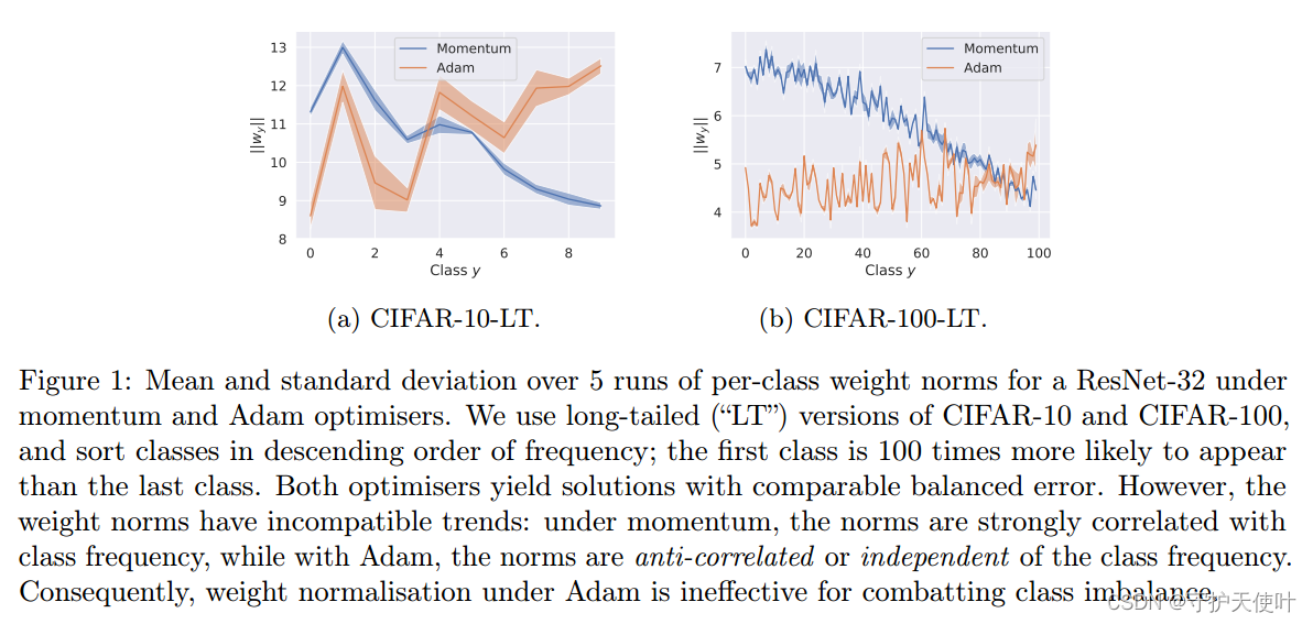
  Limitations of weight normalisation：该方式是基于权重范数$||w_y|{|}_2$与$\mathbb{P}(y)$相关，但是这十分依赖优化器的选择，从图中可以看出使用momentum和Adam优化器时的$\mathbb{P}(y)$差别极大。
  
  Limitations of loss modification：不能保证Fisher consistency。也就是说，loss最小时，balanced error也应该是最小的，但是上述两种loss都不能保证。

二、Logit adjustment for long-tail learning: a statistical view

根据之前的problem setup，我们的目标是找到一个模型$f$使得BER($f$)最小，即$f^{\ast }ϵargmi{n}_{f:\chi \to (R{)}^L}BER(f)$。下式成立：

其中${\mathbb{P}}^{bal}(y|x)\propto \mathbb{P}(x|y)\propto \frac{\mathbb{P}(y|x)}{\mathbb{P}(y)}$，假设$\mathbb{P}(y|x)\propto e^{s_y^{\ast }(x)}$，$s:\chi \to {\mathbb{R}}^L$,则（7）式变为下式：

从（8）式中可以看出，能够利用$\mathbb{P}(y)$来修正logit，从而最小化$BER(f)$。
post-hoc：训练模型估计$\mathbb{P}(y|x)$，然后按照（8）显式调整logit；
loss modification：在训练模型估计$\mathbb{P}(y|x)$时，按照（8）隐试地修正logit。

---

三、Post-hoc logit adjustment

在数据集上训练$f_y(x)=w_y^T\varphi (x)$，则（8）式就变换为下式：

（9）式相当于为每个logit加了一个偏置，这个偏置依赖于标签。$\pi$是类先验概率$\mathbb{P}(y)$的估计，$\tau$是一个超参数。

post-hoc logit adjustment相对于post-hoc weight normalization更有优势。这两种方式的调整如下图所示：

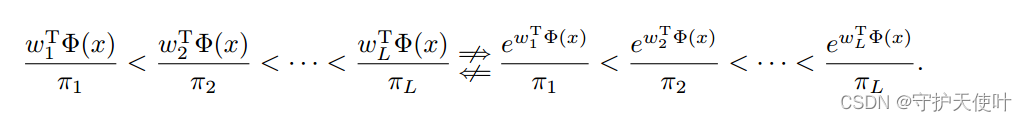
左侧为post-hoc weight normalization，是做乘法；右侧为post-hoc logit adjustment，化简之后可以成为$f_y(x)-\tau \cdot log{\pi }_y$，相当于是做加法。
对于post-hoc weight normalization，如果一个少数类得到的score是负数，其他类的score是正数，那么这个少数类只能是最小的，对于这种方法不可能让少数类获得高的score；
而对于post-hoc logit adjustment，因为做的是加法，及时score是负数，也可以通过后一项调整，给少数类很高的score，还降低了主类的score。

---

三、The logit adjusted softmax cross-entropy

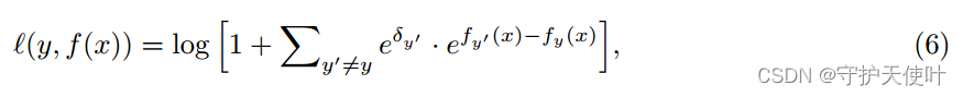
在训练时修改logit，给出基于softmax cross-entropy的loss，如下式：

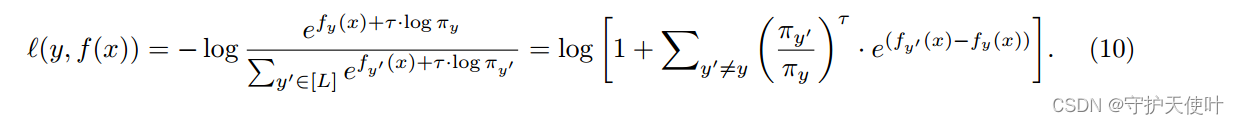
可以看做$g(x)=f_y(x)+\tau \cdot log{\pi }_y$，将$g(x)$带入了基本的softmax cross-entropy。相当于一种Post-hoc logit adjustment的方式：$argma{x}_{yϵ[L]}f(x)=argma{x}_{yϵ[L]}g(x)-\tau \cdot log{\pi }_y$。
作者给出了一般式，命名为pairwise margin loss：

该loss会使得正类和负类的margin变大。