L1 深度学习概论

2 神经网络基础作业

作业链接：吴恩达《深度学习》 - Heywhale.com

0 Jupyter Notebook基本使用

• 终端命令jupyter notebook打开Jupyter Notebook
• 单元格状态可以选择为Code或者Markdown

1 使用Numpy构建基本函数

1.1 sigomid function和np.exp()

**练习：**构建一个返回实数x的sigmoid的函数，将math.exp(x)用于指数函数

import math
def basic_sigmoid(x):
    return 1 / (1 + math.exp(-x))

basic_sigmoid(3)

• 使用math库，因为输入是实数
• 在深度学习中主要使用矩阵和向量，使用numpy更为实用

import numpy as np
def basic_sigmoid(x):
    return 1 / (1 + np.exp(-x))

basic_sigmoid(np.array([1,2,3]))

• 注意输入需要是np.array形式，使用列表报错

1.2 sigmoid gradient

练习：创建函数sigmoid_grad（）计算sigmoid函数相对于其输入x的梯度。 公式为：$sigmoid\_derivative(x)=\sigma \prime (x)=\sigma (x)(1-\sigma (x))$

import numpy as np
def sigmoid_derivative(x):
    s = 1 / (1 + np.exp(-x))
    return s * ( 1 - s)

sigmoid_derivative(np.array([1,2,3]))

1.3 reshape

np.shape：获取矩阵/向量X的形状

np.reshape()：将X重塑为其他形状

练习：实现image2vector() ,该输入采用维度为(length, height, 3)的输入，并返回维度为(length*height*3, 1)的向量。

import numpy as np
def image2vector(x):
    v = x.reshape(x.shape[0] * x.shape[1] * x.shape[2], 1)
    return v

image = np.array([[[ 0.67826139,  0.29380381],
        [ 0.90714982,  0.52835647],
        [ 0.4215251 ,  0.45017551]],

       [[ 0.92814219,  0.96677647],
        [ 0.85304703,  0.52351845],
        [ 0.19981397,  0.27417313]],

       [[ 0.60659855,  0.00533165],
        [ 0.10820313,  0.49978937],
        [ 0.34144279,  0.94630077]]])
print ("image2vector(image) = " + str(image2vector(image)))

1.4 行标准化

我们在机器学习和深度学习中使用的另一种常见技术是对数据进行标准化。 由于归一化后梯度下降的收敛速度更快，通常会表现出更好的效果。 通过归一化，也就是将x更改为$\frac{x}{\Vert x\Vert }$（将x的每个行向量除以其范数，范数为该行的所有值的平方和开根号）。

练习：执行 normalizeRows（）来标准化矩阵的行。 将此函数应用于输入矩阵x之后，x的每一行应为单位长度（即长度为1）向量。

import numpy as np
def normalizeRows(x):
    x_norm = np.linalg.norm(x, axis=1, keepdims=True)
    x = x / x_norm
    return x

x = np.array([
    [0, 3, 4],
    [1, 6, 4]])
print("normalizeRows(x) = " + str(normalizeRows(x)))

1.5 广播和softmax

练习: 使用numpy实现softmax函数。

import numpy as np
def softmax(x):
    x_exp = np.exp(x)
    x_sum = np.sum(x_exp, axis=1, keepdims=True)
    s = x_exp / x_sum
    return s

x = np.array([
    [9, 2, 5, 0, 0],
    [7, 5, 0, 0 ,0]])
print("softmax(x) = " + str(softmax(x)))

• x_sum形状为[2,1]，计算中使用了广播

• $Softmax(z_i)=\frac{e^{z_i}}{{\sum }_{c=1}^C{e}^{z_c}}$

  • $z_i$为第i个节点输出值
  • C为输出节点个数
  • 通过Softmax函数就可以将多分类的输出值转换为范围在[0, 1]和为1的概率分布

2 向量化

2.1 向量化和非向量化比较

这里在当前电脑中看不出区别

非向量化方法

import time

x1 = [9, 2, 5, 0, 0, 7, 5, 0, 0, 0, 9, 2, 5, 0, 0]
x2 = [9, 2, 2, 9, 0, 9, 2, 5, 0, 0, 9, 2, 5, 0, 0]

### CLASSIC DOT PRODUCT OF VECTORS IMPLEMENTATION ###
tic = time.process_time()
dot = 0
for i in range(len(x1)):
    dot+= x1[i]*x2[i]
toc = time.process_time()
print ("dot = " + str(dot) + "\n ----- Computation time = " + str(1000*(toc - tic)) + "ms")

### CLASSIC OUTER PRODUCT IMPLEMENTATION ###
tic = time.process_time()
outer = np.zeros((len(x1),len(x2))) # we create a len(x1)*len(x2) matrix with only zeros
for i in range(len(x1)):
    for j in range(len(x2)):
        outer[i,j] = x1[i]*x2[j]
toc = time.process_time()
print ("outer = " + str(outer) + "\n ----- Computation time = " + str(1000*(toc - tic)) + "ms")

### CLASSIC ELEMENTWISE IMPLEMENTATION ###
tic = time.process_time()
mul = np.zeros(len(x1))
for i in range(len(x1)):
    mul[i] = x1[i]*x2[i]
toc = time.process_time()
print ("elementwise multiplication = " + str(mul) + "\n ----- Computation time = " + str(1000*(toc - tic)) + "ms")

### CLASSIC GENERAL DOT PRODUCT IMPLEMENTATION ###
W = np.random.rand(3,len(x1)) # Random 3*len(x1) numpy array
tic = time.process_time()
gdot = np.zeros(W.shape[0])
for i in range(W.shape[0]):
    for j in range(len(x1)):
        gdot[i] += W[i,j]*x1[j]
toc = time.process_time()
print ("gdot = " + str(gdot) + "\n ----- Computation time = " + str(1000*(toc - tic)) + "ms")

向量化：

### VECTORIZED DOT PRODUCT OF VECTORS ###
tic = time.process_time()
dot = np.dot(x1,x2)
toc = time.process_time()
print ("dot = " + str(dot) + "\n ----- Computation time = " + str(1000*(toc - tic)) + "ms")

### VECTORIZED OUTER PRODUCT ###
tic = time.process_time()
outer = np.outer(x1,x2)
toc = time.process_time()
print ("outer = " + str(outer) + "\n ----- Computation time = " + str(1000*(toc - tic)) + "ms")

### VECTORIZED ELEMENTWISE MULTIPLICATION ###
tic = time.process_time()
mul = np.multiply(x1,x2)
toc = time.process_time()
print ("elementwise multiplication = " + str(mul) + "\n ----- Computation time = " + str(1000*(toc - tic)) + "ms")

### VECTORIZED GENERAL DOT PRODUCT ###
tic = time.process_time()
dot = np.dot(W,x1)
toc = time.process_time()
print ("gdot = " + str(dot) + "\n ----- Computation time = " + str(1000*(toc - tic)) + "ms")

• 不同于np.multiply()和* 操作符执行逐元素的乘法，np.dot()执行的是矩阵-矩阵或矩阵向量乘法

2.2 实现L1和L2损失函数

练习：实现L1损失函数的Numpy向量化版本

L1损失函数定义为：
$$L_1(\hat{y},y)=\sum _{i=0}^m|y^{(i)}-{\hat{y}}^{(i)}|$$

import numpy as np
def L1(yhat, y):
    loss = np.sum(np.abs(yhat-y))
    return loss

yhat = np.array([.9, 0.2, 0.1, .4, .9])
y = np.array([1, 0, 0, 1, 1])
print("L1 = " + str(L1(yhat,y)))

练习：实现L2损失函数的Numpy向量化版本

L2损失函数定义为：
$$L_2(\hat{y},y)=\sum _{i=0}^m(y^{(i)}-{\hat{y}}^{(i)}{)}^2$$

import numpy as np
def L2(yhat, y):
    loss = np.dot((yhat-y), (yhat-y).T)
    return loss

yhat = np.array([.9, 0.2, 0.1, .4, .9])
y = np.array([1, 0, 0, 1, 1])
print("L2 = " + str(L2(yhat,y)))

• 注意这里平方使用的是矩阵与转置矩阵的np.dot()乘法

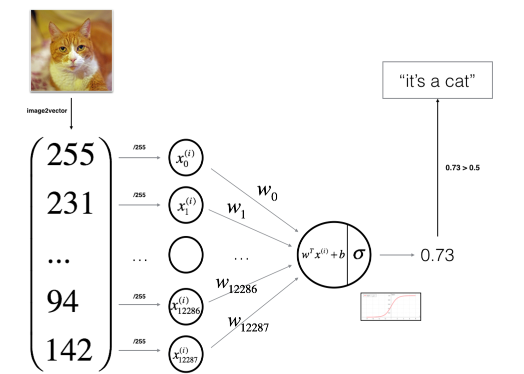
3 用神经网络思想实现Logistic回归

整体结构如下所示：

3.1 导入安装包

import numpy as np
import matplotlib.pyplot as plt
import h5py
import scipy
from PIL import Image
from scipy import ndimage
from lr_utils import load_dataset

%matplotlib inline

• lr_utils为写好的加载数据集的python文件

3.2 问题概述

问题说明：你将获得一个包含以下内容的数据集（“data.h5”）：

• 标记为cat（y = 1）或非cat（y = 0）的m_train训练图像集
• 标记为cat或non-cat的m_test测试图像集
• 图像维度为（num_px，num_px，3），其中3表示3个通道（RGB）。 因此，每个图像都是正方形（高度= num_px）和（宽度= num_px）。

构建一个简单的图像识别算法，该算法可以将图片正确分类为猫和非猫。
加载并查看数据：

train_set_x_orig, train_set_y, test_set_x_orig, test_set_y, classes = load_dataset()

# Example of a picture
index = 5
plt.imshow(train_set_x_orig[index])
print ("y = " + str(train_set_y[:, index]) + ", it's a '" + classes[np.squeeze(train_set_y[:, index])].decode("utf-8") +  "' picture.")

m_train = train_set_x_orig.shape[0]
m_test = test_set_x_orig.shape[0]
num_px = train_set_x_orig.shape[1]

print ("Number of training examples: m_train = " + str(m_train))
print ("Number of testing examples: m_test = " + str(m_test))
print ("Height/Width of each image: num_px = " + str(num_px))
print ("Each image is of size: (" + str(num_px) + ", " + str(num_px) + ", 3)")
print ("train_set_x shape: " + str(train_set_x_orig.shape))
print ("train_set_y shape: " + str(train_set_y.shape))
print ("test_set_x shape: " + str(test_set_x_orig.shape))
print ("test_set_y shape: " + str(test_set_y.shape))

获得训练集结果：

训练集数量：m_train = 209
测试集数量：m_test = 50
每个图像的高度/宽度：num_px = 64
每个图像的大小：（64，64，3）
train_set_x维度：（209、64、64、3）
trainsety维度：（1，209）
test_set_x维度：（50、64、64、3）
test_set_y维度：（1，50）

重组数据大小：

# Reshape the training and test examples

train_set_x_flatten = train_set_x_orig.reshape(train_set_x_orig.shape[0], -1).T
test_set_x_flatten = test_set_x_orig.reshape(test_set_x_orig.shape[0], -1).T

print ("train_set_x_flatten shape: " + str(train_set_x_flatten.shape))
print ("train_set_y shape: " + str(train_set_y.shape))
print ("test_set_x_flatten shape: " + str(test_set_x_flatten.shape))
print ("test_set_y shape: " + str(test_set_y.shape))
print ("sanity check after reshaping: " + str(train_set_x_flatten[0:5,0]))

重组后的结果：

train_set_x_flatten维度：（12288，209）
trainsety维度：（1，209）
test_set_x_flatten维度：（12288，50）
test_set_y维度：（1，50）
重塑后的检查维度：[17 31 56 22 33]

由于图片数据为R、G、B三个通道0到255值，因此进行标准化：

train_set_x = train_set_x_flatten/255.
test_set_x = test_set_x_flatten/255.

• 预处理数据常见步骤：
  • 获得数据的尺寸和维度
  • 重塑数据集
  • 标准化数据

3.3 搭建一般架构

搭建步骤如下所示：

1. 初始化模型参数
2. 通过最小化损失函数来学习模型的参数
3. 使用学习到的参数进行预测
4. 分析结果并得出结论

辅助函数编写：

# GRADED FUNCTION: sigmoid

def sigmoid(z):
    """
    Compute the sigmoid of z

    Arguments:
    z -- A scalar or numpy array of any size.

    Return:
    s -- sigmoid(z)
    """

    s = 1 / (1 + np.exp(-z))
    
    return s

初始化参数：

def initialize_with_zeros(dim):
    """
    This function creates a vector of zeros of shape (dim, 1) for w and initializes b to 0.
    
    Argument:
    dim -- size of the w vector we want (or number of parameters in this case)
    
    Returns:
    w -- initialized vector of shape (dim, 1)
    b -- initialized scalar (corresponds to the bias)
    """
    
    w = np.zeros((dim, 1))
    b = 0

    assert(w.shape == (dim, 1))
    assert(isinstance(b, float) or isinstance(b, int))
    
    return w, b

前向传播函数

1. 得到X
2. 计算A = σ(w^TX + b)
3. 计算损失函数

# GRADED FUNCTION: propagate

def propagate(w, b, X, Y):
    """
    Implement the cost function and its gradient for the propagation explained above

    Arguments:
    w -- weights, a numpy array of size (num_px * num_px * 3, 1)
    b -- bias, a scalar
    X -- data of size (num_px * num_px * 3, number of examples)
    Y -- true "label" vector (containing 0 if non-cat, 1 if cat) of size (1, number of examples)

    Return:
    cost -- negative log-likelihood cost for logistic regression
    dw -- gradient of the loss with respect to w, thus same shape as w
    db -- gradient of the loss with respect to b, thus same shape as b
    """
    m = X.shape[1]
    
    # FORWARD PROPAGATION (FROM X TO COST)
    A = sigmoid(np.dot(w.T, X) + b)            # compute activation
    cost = -1 / m * np.sum(Y * np.log(A) + (1 - Y) * np.log(1 - A))         # compute cost
    
    # BACKWARD PROPAGATION (TO FIND GRAD)
    dw = 1 / m * np.dot(X, (A - Y).T)
    db = 1 / m * np.sum(A - Y)
    assert(dw.shape == w.shape)
    assert(db.dtype == float)
    cost = np.squeeze(cost)
    assert(cost.shape == ())
    
    grads = {"dw": dw,
             "db": db}
    
    return grads, cost

优化函数：

1. 初始化参数
2. 计算损失函数及其梯度
3. 使用梯度下降法更新参数

# GRADED FUNCTION: optimize

def optimize(w, b, X, Y, num_iterations, learning_rate, print_cost = False):
    """
    This function optimizes w and b by running a gradient descent algorithm
    
    Arguments:
    w -- weights, a numpy array of size (num_px * num_px * 3, 1)
    b -- bias, a scalar
    X -- data of shape (num_px * num_px * 3, number of examples)
    Y -- true "label" vector (containing 0 if non-cat, 1 if cat), of shape (1, number of examples)
    num_iterations -- number of iterations of the optimization loop
    learning_rate -- learning rate of the gradient descent update rule
    print_cost -- True to print the loss every 100 steps
    
    Returns:
    params -- dictionary containing the weights w and bias b
    grads -- dictionary containing the gradients of the weights and bias with respect to the cost function
    costs -- list of all the costs computed during the optimization, this will be used to plot the learning curve.

    """
    
    costs = []
    
    for i in range(num_iterations):
        
        
        # Cost and gradient calculation
        grads, cost = propagate(w, b, X, Y)
        
        # Retrieve derivatives from grads
        dw = grads["dw"]
        db = grads["db"]
        
        # update rule
        w = w - learning_rate * dw
        b = b - learning_rate * db
        
        # Record the costs
        if i % 100 == 0:
            costs.append(cost)
        
        # Print the cost every 100 training examples
        if print_cost and i % 100 == 0:
            print ("Cost after iteration %i: %f" %(i, cost))
    
    params = {"w": w,
              "b": b}
    
    grads = {"dw": dw,
             "db": db}
    
    return params, grads, costs

练习： 上一个函数将输出学习到的w和b。 我们能够使用w和b来预测数据集X的标签。实现predict（）函数。 预测分类有两个步骤：

1. 计算$\hat{Y}=A=\sigma (w^{T}X+b)$
2. 将a的项转换为0（如果A <= 0.5）或1（如果A > 0.5），并将预测结果存储在向量“ Y_prediction”中。 如果愿意，可以在for循环中使用if / else语句。

# GRADED FUNCTION: predict

def predict(w, b, X):
    '''
    Predict whether the label is 0 or 1 using learned logistic regression parameters (w, b)
    
    Arguments:
    w -- weights, a numpy array of size (num_px * num_px * 3, 1)
    b -- bias, a scalar
    X -- data of size (num_px * num_px * 3, number of examples)
    
    Returns:
    Y_prediction -- a numpy array (vector) containing all predictions (0/1) for the examples in X
    '''
    
    m = X.shape[1]
    Y_prediction = np.zeros((1,m))
    w = w.reshape(X.shape[0], 1)
    
    # Compute vector "A" predicting the probabilities of a cat being present in the picture
    ### START CODE HERE ### (≈ 1 line of code)
    A = sigmoid(np.dot(w.T, X) + b)
    ### END CODE HERE ###

    for i in range(A.shape[1]):
        
        # Convert probabilities A[0,i] to actual predictions p[0,i]
        ### START CODE HERE ### (≈ 4 lines of code)
        if A[0, i] <= 0.5:
            Y_prediction[0, i] = 0
        else:
            Y_prediction[0, i] = 1
        ### END CODE HERE ###
    
    assert(Y_prediction.shape == (1, m))
    
    return Y_prediction

3.4 合并功能到模型

练习： 实现模型功能，使用以下符号：

• Y_prediction对测试集的预测
• Y_prediction_train对训练集的预测
• w，损失，optimize（）输出的梯度

# GRADED FUNCTION: model

def model(X_train, Y_train, X_test, Y_test, num_iterations = 2000, learning_rate = 0.5, print_cost = False):
    """
    Builds the logistic regression model by calling the function you've implemented previously
    
    Arguments:
    X_train -- training set represented by a numpy array of shape (num_px * num_px * 3, m_train)
    Y_train -- training labels represented by a numpy array (vector) of shape (1, m_train)
    X_test -- test set represented by a numpy array of shape (num_px * num_px * 3, m_test)
    Y_test -- test labels represented by a numpy array (vector) of shape (1, m_test)
    num_iterations -- hyperparameter representing the number of iterations to optimize the parameters
    learning_rate -- hyperparameter representing the learning rate used in the update rule of optimize()
    print_cost -- Set to true to print the cost every 100 iterations
    
    Returns:
    d -- dictionary containing information about the model.
    """
    
    
    # initialize parameters with zeros
    w, b = initialize_with_zeros(X_train.shape[0])

    # Gradient descent
    parameters, grads, costs = optimize(w, b, X_train, Y_train, num_iterations, learning_rate, print_cost)
    
    # Retrieve parameters w and b from dictionary "parameters"
    w = parameters["w"]
    b = parameters["b"]
    
    # Predict test/train set examples 
    Y_prediction_test = predict(w, b, X_test)
    Y_prediction_train = predict(w, b, X_train)

    # Print train/test Errors
    print("train accuracy: {} %".format(100 - np.mean(np.abs(Y_prediction_train - Y_train)) * 100))
    print("test accuracy: {} %".format(100 - np.mean(np.abs(Y_prediction_test - Y_test)) * 100))

    
    d = {"costs": costs,
         "Y_prediction_test": Y_prediction_test, 
         "Y_prediction_train" : Y_prediction_train, 
         "w" : w, 
         "b" : b,
         "learning_rate" : learning_rate,
         "num_iterations": num_iterations}
    
    return d

使用如下代码进行训练：

d = model(train_set_x, train_set_y, test_set_x, test_set_y, num_iterations = 2000, learning_rate = 0.005, print_cost = True)

使用下面代码可以查看测试集上的单张图片预测情况

# Example of a picture that was wrongly classified.
index = 1
plt.imshow(test_set_x[:,index].reshape((num_px, num_px, 3)))
print ("y = " + str(test_set_y[0,index]) + ", you predicted that it is a \"" + classes[int(d["Y_prediction_test"][0,index])].decode("utf-8") +  "\" picture.")

绘制损失函数：

# Plot learning curve (with costs)
costs = np.squeeze(d['costs'])
plt.plot(costs)
plt.ylabel('cost')
plt.xlabel('iterations (per hundreds)')
plt.title("Learning rate =" + str(d["learning_rate"]))
plt.show()

3.5 学习率

学习率α决定我们更新参数的速度

• 如果学习率太大，可能会超出最佳值
• 如果太小，将需要更多的迭代才能收敛到最佳值

不同学习率比较及损失函数绘制：

learning_rates = [0.01, 0.001, 0.0001]
models = {}
for i in learning_rates:
    print ("learning rate is: " + str(i))
    models[str(i)] = model(train_set_x, train_set_y, test_set_x, test_set_y, num_iterations = 1500, learning_rate = i, print_cost = False)
    print ('\n' + "-------------------------------------------------------" + '\n')

for i in learning_rates:
    plt.plot(np.squeeze(models[str(i)]["costs"]), label= str(models[str(i)]["learning_rate"]))

plt.ylabel('cost')
plt.xlabel('iterations')

legend = plt.legend(loc='upper center', shadow=True)
frame = legend.get_frame()
frame.set_facecolor('0.90')
plt.show()

• 不同的学习率会带来不同的损失，因此会有不同的预测结果
• 如果学习率太大（0.01），则成本可能会上下波动，它甚至可能会发散
• 较低的损失并不意味着模型效果很好。当训练精度比测试精度高很多时，就会发生过拟合情况
• 在深度学习中，通常建议：
  • 选择好能最小化损失函数的学习率
  • 如果模型过度拟合，使用其他方法来减少过度拟合

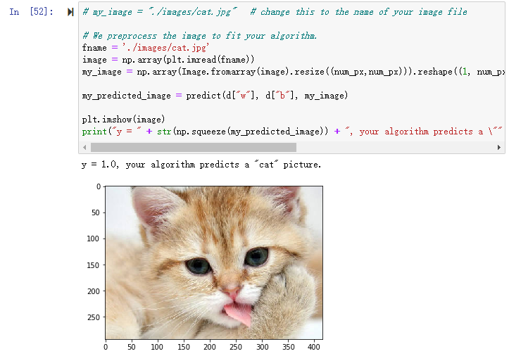
3.6 使用自己的图像进行测试

将fname路径修改为自己的图片路径

# my_image = "./images/cat.jpg"   # change this to the name of your image file 

# We preprocess the image to fit your algorithm.
fname = './images/cat.jpg'
image = np.array(plt.imread(fname))
my_image = np.array(Image.fromarray(image).resize((num_px,num_px))).reshape((1, num_px*num_px*3)).T

my_predicted_image = predict(d["w"], d["b"], my_image)

plt.imshow(image)
print("y = " + str(np.squeeze(my_predicted_image)) + ", your algorithm predicts a \"" + classes[int(np.squeeze(my_predicted_image)),].decode("utf-8") +  "\" picture.")

运行结果如下所示：

• 原版教程中scipy因为版本更新原因没有了scipy.misc方法，上面代码中my_image = scipy.misc.imresize(image, size=(num_px,num_px)).reshape((1, num_px*num_px*3)).T替换为my_image = np.array(Image.fromarray(image).resize((num_px,num_px))).reshape((1, num_px*num_px*3)).T