机器学习——时间序列模型
文章目录1. 基本概念2. 基本操作2.1 平稳性检测2.2 白噪声检验3. 模式识别4. 建模步骤平稳性检验白噪声检验模型识别参数计算模型优化模型预测模型名称秒是平滑法削弱短期随机波动对序列的影响,序列插值分布均匀趋势拟合法把时间作为自变量,相应序列观察值作为因变量,简历回归模型组合模型法受长期趋势(T)、季节变动(S)、周期变动(C)和不规则变动(ε)四个因素影响组合模型(1)加法模型:T+S
| 模型名称 | 描述 |
|---|---|
| 平滑法 | 削弱短期随机波动对序列的影响,序列插值分布均匀 |
| 趋势拟合法 | 把时间作为自变量,相应序列观察值作为因变量,简历回归模型 |
| 组合模型法 | 受长期趋势(T)、季节变动(S)、周期变动(C)和不规则变动(ε)四个因素影响 |
| 组合模型 | (1)加法模型: T + S + C + ϵ T+S+C+\epsilon T+S+C+ϵ (2)乘法模型: T S C ϵ T SC\epsilon TSCϵ |
常见时间序列模型
| 模型名称 | 描述 |
|---|---|
| AR模型 | 考虑历史数据的影响,以过往数据为自变量, X t X_t Xt为因变量建立线性回归模型。 X t = ϕ 0 + ϕ 1 x t − 1 + ⋯ + ϕ p x t − p X_t=\phi_0+\phi_1 x_{t-1}+\cdots+\phi_p x_{t-p} Xt=ϕ0+ϕ1xt−1+⋯+ϕpxt−p |
| MA模型 | 忽略历史数据影响,建立于前q期随机扰动 ϵ t − 1 , ⋯ , ϵ t − q \epsilon_{t-1},\cdots,\epsilon_{t-q} ϵt−1,⋯,ϵt−q的线性回归模型 X t = μ + ϵ t − θ 1 ϵ t − 1 − ⋯ − θ q ϵ t − q X_t=\mu+\epsilon_t-\theta_1 \epsilon_{t-1}-\cdots-\theta_q \epsilon_{t-q} Xt=μ+ϵt−θ1ϵt−1−⋯−θqϵt−q |
| ARMA模型 | 结合考虑AR、MA模型,综合考虑它们的影响 |
| ARIMA模型 | 针对非平稳序列。将非平稳转化为平稳后拟合操作 |
1. 基本概念
白噪声序列: 数据随机分布,没有规律。
平稳非白噪声序列
非平稳序列: 可以利用差分法转换为平稳非白噪声序列
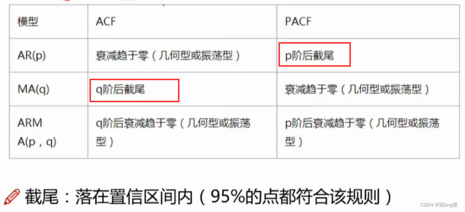
截尾: 拖尾指序列以指数率单调递减或震荡衰减
拖尾: 截尾指序列从某个时点变得非常小

1.1 自相关函数ACF(autocorrelation function)
- 自相关函数反映了同一序列在不同时序的取值之间的相关性。
- 公式:
A C F ( k ) = ρ k = C o v ( y t , y t − k ) V a r ( y t ) ACF(k) = \rho_k=\frac{Cov(y_t,y_{t-k})}{Var(y_t)} ACF(k)=ρk=Var(yt)Cov(yt,yt−k)
其中, ρ k ∈ [ − 1 , 1 ] \rho_k \in[-1,1] ρk∈[−1,1]
1.2 偏自相关函数PACF(partial autocorrelation function)
- 剔除了中间k-1个随机变量 x ( t − 1 ) , x ( t − 2 ) , ⋯ , x ( t − k + 1 ) x(t-1),x(t-2),\cdots,x(t-k+1) x(t−1),x(t−2),⋯,x(t−k+1)的干扰后 x ( t − k ) x(t-k) x(t−k)对 x ( t ) x(t) x(t)影响的相关程度
- PACF是严格两个变量之间的相关性。
2. 常见模型
2.1 自回归模型(AR)
定义:
-
描述当前值与历史值之间的关系。利用历史数据对自身进行预测
-
P阶自回归过程,即当前值与 t − p , t − p + 1 , ⋯ , t − 1 t-p,t-p+1,\cdots,t-1 t−p,t−p+1,⋯,t−1相关(P)。
y t = μ + ∑ i = 1 p γ i y t − i + ϵ t y_t=\mu+\sum_{i=1}^{p} \gamma_i y_{t-i} + \epsilon_t yt=μ+i=1∑pγiyt−i+ϵt
其中, y t y_t yt是当前值, μ \mu μ是常数项,P是阶数, γ i \gamma_i γi是自相关系数, ϵ \epsilon ϵ是误差。 -
参数:P(自回归阶数)
注意
- 必须具有平稳性
- 必须具有自相关性,自相关系数需要大于等于0.5.
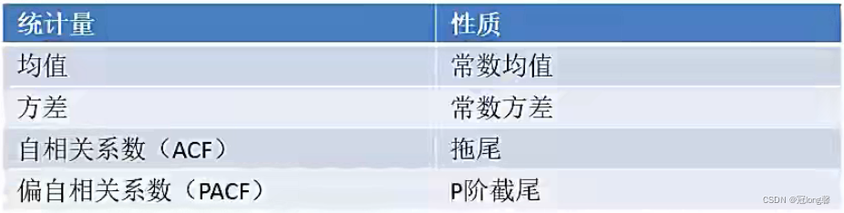
模型识别
2.2 移动平均模型(MA)
定义
-
移动平均模型是自回归模型中误差项的累加
-
q阶移动模型公式(Q):
y t = μ + ϵ t + ∑ i = 1 q θ i ϵ t − i y_t = \mu + \epsilon_t + \sum_{i=1}^{q} \theta_i \epsilon_{t-i} yt=μ+ϵt+i=1∑qθiϵt−i -
移动平均法能有效地消除预测中的随机波动
-
参数:Q(移动平均阶数)
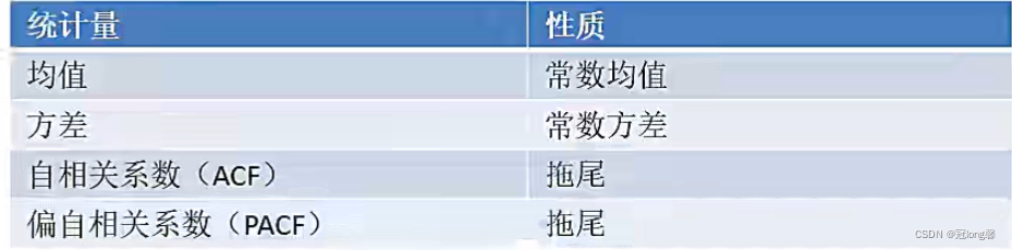
模型识别

2.3 自回归移动平均模型(ARMA)
定义
-
自回归与移动平均的结合
-
公式定义为(P,Q):
y t = μ + ∑ i = 1 p γ i y t − i + ϵ t + ∑ i = 1 q θ i ϵ t − i y_t = \mu + \sum_{i=1}^{p} \gamma_i y_{t-i} + \epsilon_t + \sum_{i=1}^{q} \theta_i \epsilon_{t-i} yt=μ+i=1∑pγiyt−i+ϵt+i=1∑qθiϵt−i -
参数:P(自回归阶数),Q(移动平均阶数)
模型识别
2.4 差分自回归移动平均模型(ARIMA)
对于ARIMA模型,我们需要指定三个参数(P, D, Q),分别表示P阶自回归模型,D阶差分和Q阶移动平均模型。
定义:
- 参数:(P, D, Q),分别表示P阶自回归模型,D阶差分和Q阶移动平均模型。
- 原理:将非平稳时间序列转换为平稳时间序列,然后将因变量对其滞后值和其随机误差的滞后值进行回归建模。
4. 建模步骤
4.1 平稳性检验
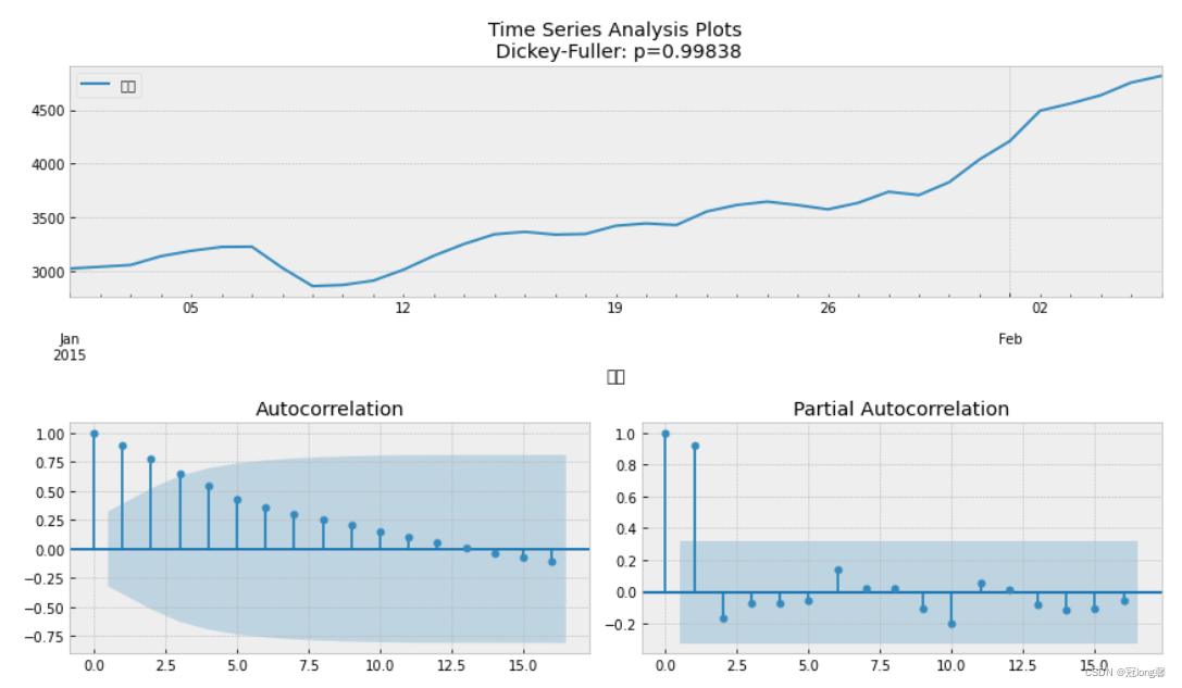
4.1.1 时序图、自相关图、偏自相关图
def tsplot(y,lags=None,figsize=(12,7),style='bmh'):
    '''
    Plot time series, its ACF and PACF, calculate Dickey-Fuller test
    y:timeseries
    lags:how many lags to include in ACF,PACF calculation
    '''
#     if not isinstance(y, pd.Series):
#         y = pd.Series(y)
    with plt.style.context(style):
        fig = plt.figure(figsize=figsize)
        layout=(2,2)
        ts_ax = plt.subplot2grid(layout, (0,0), colspan=2)
        acf_ax = plt.subplot2grid(layout, (1,0))
        pacf_ax = plt.subplot2grid(layout, (1,1))

        y.plot(ax=ts_ax)
        p_value = sm.tsa.stattools.adfuller(y)[1]
        ts_ax.set_title('Time Series Analysis Plots\n Dickey-Fuller: p={0:.5f}'.format(p_value))
        smt.graphics.plot_acf(y,lags=lags, ax=acf_ax)
        smt.graphics.plot_pacf(y,lags=lags, ax=pacf_ax)
        plt.tight_layout()
tsplot(data)
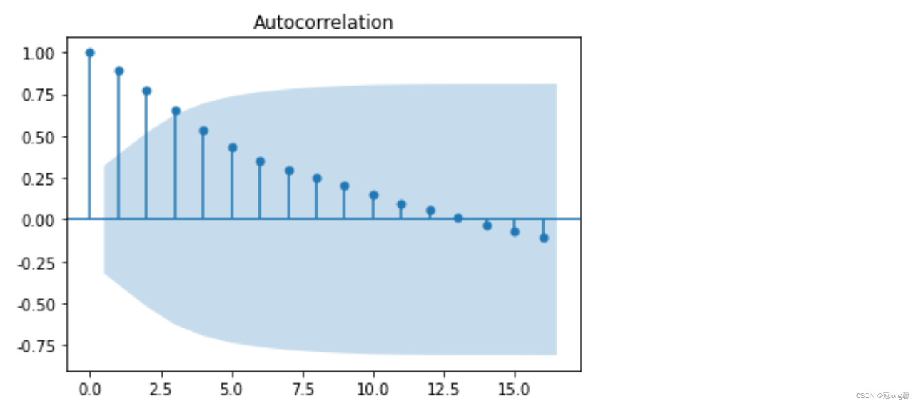
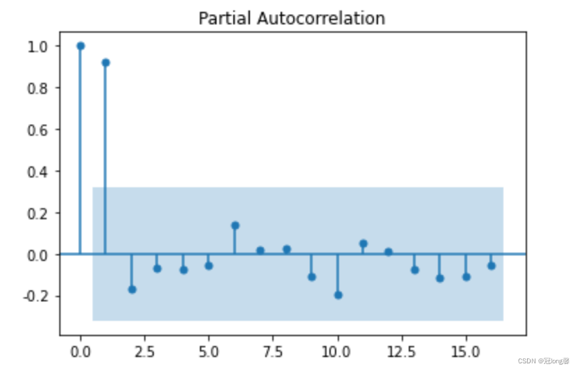
4.1.2 自相关、偏自相关图
根据自相关图,判断“拖尾”、“截尾”。
from statsmodels.graphics.tsaplots import plot_acf
plot_acf(data).show()
from statsmodels.graphics.tsaplots import plot_pacf
plot_pacf(data).show()
4.1.3 单位根检验
采用单位根法检验,当单位根大于等于0.05时,表示数据为非平稳序列。
from statsmodels.tsa.stattools import adfuller as ADF
print('原始序列数据的ADF检测结果为:')
print(ADF(data['销量']))
# 返回值依次为: adf, pvalue(单位根,>=0.05就是非平稳序列)
原始序列数据的ADF检测结果为:
(1.813771015094526, 0.9983759421514264, 10, 26, {‘1%’: -3.7112123008648155, ‘5%’: -2.981246804733728, ‘10%’: -2.6300945562130176}, 299.4698986602418)
4.1.4 差分运算
若序列为非平稳序列,则需要转换为平稳序列计算
(1)差分运算
- P阶差分
相距一期的两个序列之间的减法运算称为1阶差分运算
将1阶差分运算的结果再做一次差分运算则称为2阶差分运算 - K步差分
相距k期的两个序列值之间的减法运算称为k步差分运算
1. 差分运算
D_data = data.diff().dropna()    # 一阶一步差分,并去除NA
D_data.columns = ['sale diff']
2. 差分结果检验
对差分结果进行相同的平稳性检验,当单位根值小于等于0.05时,表示已经转换为平稳序列。
# 自相关图
plot_acf(D_data).show()
# 偏自相关图
plot_pacf(D_data).show()
# 单位根值
print('原始序列数据进行一次一步差分的ADF检测结果为:')
print(ADF(D_data['sale diff']))
原始序列数据进行一次一步差分的ADF检测结果为:
(-3.1560562366723537, 0.022673435440048798, 0, 35, {‘1%’: -3.6327426647230316, ‘5%’: -2.9485102040816327, ‘10%’: -2.6130173469387756}, 287.5909090780334)
4.2 白噪声检验
from statsmodels.stats.diagnostic import acorr_ljungbox
print('差分序列的白噪声检验结果:')
print(acorr_ljungbox(D_data,lags=1))   # 返回统计量与p值,当p <= 0.05 时,不是白噪音
差分序列的白噪声检验结果:
(array([11.30402222]), array([0.00077339]))
4.3 模型选择(p,q,d)
AR, MA模型
通过ACF, PACF截尾开始阶数确定p, q参数值。
- AR§:PACF上截尾,ACF趋近于0
- MA(Q):ACF上截尾,PACF趋近于0
采用BIC矩阵,找到最小值对应的p, q值。并以此为参数选择下述三个模型:
4.3.1 AIC与BIC
AIC:赤池信息准则(Akaike information Criterion)
A
I
C
=
2
k
−
2
ln
(
L
)
AIC = 2k-2\ln(L)
AIC=2k−2ln(L)
BIC:贝叶斯信息准则(Bayesian information Criterion)
B
I
C
=
k
ln
(
n
)
−
2
ln
(
L
)
BIC = k\ln(n)-2\ln(L)
BIC=kln(n)−2ln(L)
其中,k为模型参数个数,n为样本数量,L为似然函数。
from statsmodels.tsa.arima_model import ARIMA
# 定阶
# data['销量']=data['销量'].astype(float)
pmax = int(len(D_data)/10)
qmax = int(len(D_data)/10)
bic_matrix = [] # BIC矩阵
for p in range(pmax+1):
tmp = []
for q in range(qmax+1):
try: # 部分报错,跳过
tmp.append(ARIMA(data,(p,1,q)).fit().bic)
except:
tmp.append(None)
bic_matrix.append(tmp)
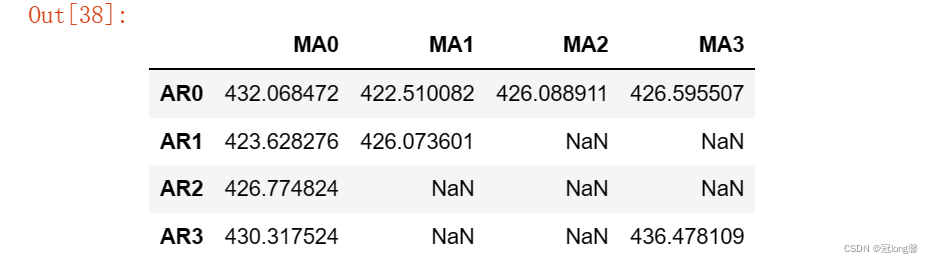
bic_matrix = pd.DataFrame(bic_matrix)
bic_matrix.index = ['AR{}'.format(i) for i in range(pmax+1)]
bic_matrix.columns = ['MA{}'.format(i) for i in range(qmax+1)]
bic_matrix = bic_matrix[bic_matrix.columns].astype(float)
p,q = bic_matrix.stack().idxmin()
print('最小BIC对应的p,q值:%s, %s'%(p,q))
最小BIC对应的p,q值:0, 1
import seaborn as sns
fig, ax = plt.subplots(figsize = (10,8))
ax = sns.heatmap(bic_matrix,
                mask = bic_matrix.isnull(),
                ax = ax,
                annot = True,
                fmt='.2f')
ax.set_title('BIC')

result = smt.arma_order_select_ic(data, ic=['aic', 'bic'], trend='nc', max_ar=4, max_ma=4)
{‘aic’: 0 1 2 3 4
0 NaN 668.212060 627.212365 590.498371 565.724666
1 472.121781 442.706792 444.414985 441.613728 442.640421
2 449.878586 443.006993 445.873538 443.364868 445.454087
3 452.992514 441.894814 443.613869 449.670033 442.185777
4 454.442210 443.477934 445.326246 445.745273 445.296295,
‘bic’: 0 1 2 3 4
0 NaN 671.433896 632.045119 596.942043 573.779256
1 475.343616 447.539546 450.858657 449.668317 452.305928
2 454.711339 449.450664 453.928128 453.030375 456.730513
3 459.436186 449.949403 453.279376 460.946459 455.073120
4 462.496800 453.143442 456.602672 458.632617 459.794557,
‘aic_min_order’: (1, 3),
‘bic_min_order’: (1, 1)}
由此可以选择MA模型,或者p =0, q =1的ARMA模型。可以将做完差分的数据带入平稳模型或者将原数据带入非平稳模型,并设置阶数。
4.3.2 模型稳定性检验
模型残差检验
- ARIMA的残差是否是平均值为0且方差为常数的正太分布
- QQ图:线性即正太分布
4.4 模型预测
model = ARIMA(data, (p,1,q)).fit()
print('模型报告为:\n', model.summary2())
print('未来5天的预测结果、准确误差及置信区间:\n',model.forecast(5))


CSDN联合极客时间,共同打造面向开发者的精品内容学习社区,助力成长!
更多推荐


 7
7 0
0- 0


 已为社区贡献1条内容

所有评论(0)