
PyTorch入门(二)搭建MLP模型实现分类任务
本文将会介绍如何使用PyTorch来搭建简单的MLP(Multi-layer Perceptron,多层感知机)模型,来实现二分类及多分类任务。
本文是PyTorch入门的第二篇文章,后续将会持续更新,作为PyTorch系列文章。
本文将会介绍如何使用PyTorch来搭建简单的MLP(Multi-layer Perceptron,多层感知机)模型,来实现二分类及多分类任务。
数据集介绍
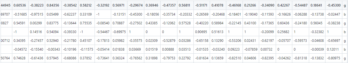
二分类数据集为ionosphere.csv(电离层数据集),是UCI机器学习数据集中的经典二分类数据集。它一共有351个观测值,34个自变量,1个因变量(类别),类别取值为g(good)和b(bad)。在ionosphere.csv文件中,共351行,前34列作为自变量(输入的X),最后一列作为类别值(输出的y)。
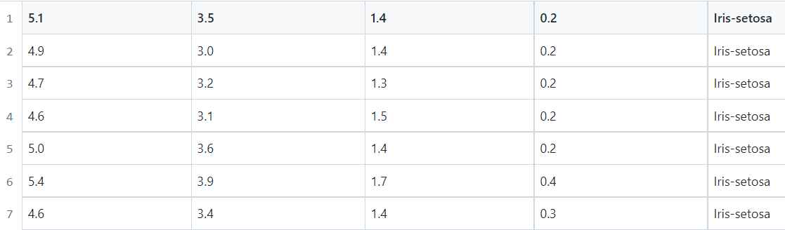
多分类数据集为iris.csv(鸢尾花数据集),是UCI机器学习数据集中的经典多分类数据集。它一共有150个观测值,4个自变量(萼片长度,萼片宽度,花瓣长度,花瓣宽度),1个因变量(类别),类别取值为Iris-setosa,Iris-versicolour,Iris-virginica。在iris.csv文件中,共150行,前4列作为自变量(输入的X),最后一列作为类别值(输出的y)。前几行数据如下图:
分类模型流程
使用PyTorch构建神经网络模型来解决分类问题的基本流程如下:
其中加载数据集和划分数据集为数据处理部分,构建模型和选择损失函数及优化器为创建模型部分,模型训练的目标是选择合适的优化器及训练步长使得损失函数的值很小,模型预测是在模型测试集或新数据上的预测。
二分类模型
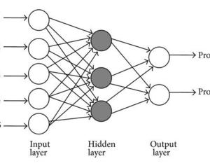
使用PyTorch构建MLP模型来实现二分类任务,模型结果图如下:
实现MLP模型的Python代码如下:
# -*- coding: utf-8 -*-
# pytorch mlp for binary classification
from numpy import vstack
from pandas import read_csv
from sklearn.preprocessing import LabelEncoder
from sklearn.metrics import accuracy_score
from torch import Tensor
from torch.optim import SGD
from torch.utils.data import Dataset, DataLoader, random_split
from torch.nn import Linear, ReLU, Sigmoid, Module, BCELoss
from torch.nn.init import kaiming_uniform_, xavier_uniform_


# dataset definition
class CSVDataset(Dataset):
    # load the dataset
    def __init__(self, path):
        # load the csv file as a dataframe
        df = read_csv(path, header=None)
        # store the inputs and outputs
        self.X = df.values[:, :-1]
        self.y = df.values[:, -1]
        # ensure input data is floats
        self.X = self.X.astype('float32')
        # label encode target and ensure the values are floats
        self.y = LabelEncoder().fit_transform(self.y)
        self.y = self.y.astype('float32')
        self.y = self.y.reshape((len(self.y), 1))

    # number of rows in the dataset
    def __len__(self):
        return len(self.X)

    # get a row at an index
    def __getitem__(self, idx):
        return [self.X[idx], self.y[idx]]

    # get indexes for train and test rows
    def get_splits(self, n_test=0.3):
        # determine sizes
        test_size = round(n_test * len(self.X))
        train_size = len(self.X) - test_size
        # calculate the split
        return random_split(self, [train_size, test_size])


# model definition
class MLP(Module):
    # define model elements
    def __init__(self, n_inputs):
        super(MLP, self).__init__()
        # input to first hidden layer
        self.hidden1 = Linear(n_inputs, 10)
        kaiming_uniform_(self.hidden1.weight, nonlinearity='relu')
        self.act1 = ReLU()
        # second hidden layer
        self.hidden2 = Linear(10, 8)
        kaiming_uniform_(self.hidden2.weight, nonlinearity='relu')
        self.act2 = ReLU()
        # third hidden layer and output
        self.hidden3 = Linear(8, 1)
        xavier_uniform_(self.hidden3.weight)
        self.act3 = Sigmoid()

    # forward propagate input
    def forward(self, X):
        # input to first hidden layer
        X = self.hidden1(X)
        X = self.act1(X)
        # second hidden layer
        X = self.hidden2(X)
        X = self.act2(X)
        # third hidden layer and output
        X = self.hidden3(X)
        X = self.act3(X)
        return X


# prepare the dataset
def prepare_data(path):
    # load the dataset
    dataset = CSVDataset(path)
    # calculate split
    train, test = dataset.get_splits()
    # prepare data loaders
    train_dl = DataLoader(train, batch_size=32, shuffle=True)
    test_dl = DataLoader(test, batch_size=1024, shuffle=False)
    return train_dl, test_dl


# train the model
def train_model(train_dl, model):
    # define the optimization
    criterion = BCELoss()
    optimizer = SGD(model.parameters(), lr=0.01, momentum=0.9)
    # enumerate epochs
    for epoch in range(100):
        # enumerate mini batches
        for i, (inputs, targets) in enumerate(train_dl):
            # clear the gradients
            optimizer.zero_grad()
            # compute the model output
            yhat = model(inputs)
            # calculate loss
            loss = criterion(yhat, targets)
            # credit assignment
            loss.backward()
            print("epoch: {}, batch: {}, loss: {}".format(epoch, i, loss.data))
            # update model weights
            optimizer.step()


# evaluate the model
def evaluate_model(test_dl, model):
    predictions, actuals = [], []
    for i, (inputs, targets) in enumerate(test_dl):
        # evaluate the model on the test set
        yhat = model(inputs)
        # retrieve numpy array
        yhat = yhat.detach().numpy()
        actual = targets.numpy()
        actual = actual.reshape((len(actual), 1))
        # round to class values
        yhat = yhat.round()
        # store
        predictions.append(yhat)
        actuals.append(actual)
    predictions, actuals = vstack(predictions), vstack(actuals)
    # calculate accuracy
    acc = accuracy_score(actuals, predictions)
    return acc


# make a class prediction for one row of data
def predict(row, model):
    # convert row to data
    row = Tensor([row])
    # make prediction
    yhat = model(row)
    # retrieve numpy array
    yhat = yhat.detach().numpy()
    return yhat


# prepare the data
path = './data/ionosphere.csv'
train_dl, test_dl = prepare_data(path)
print(len(train_dl.dataset), len(test_dl.dataset))
# define the network
model = MLP(34)
print(model)
# train the model
train_model(train_dl, model)
# evaluate the model
acc = evaluate_model(test_dl, model)
print('Accuracy: %.3f' % acc)
# make a single prediction (expect class=1)
row = [1, 0, 0.99539, -0.05889, 0.85243, 0.02306, 0.83398, -0.37708, 1, 0.03760, 0.85243, -0.17755, 0.59755, -0.44945,
       0.60536, -0.38223, 0.84356, -0.38542, 0.58212, -0.32192, 0.56971, -0.29674, 0.36946, -0.47357, 0.56811, -0.51171,
       0.41078, -0.46168, 0.21266, -0.34090, 0.42267, -0.54487, 0.18641, -0.45300]
yhat = predict(row, model)
print('Predicted: %.3f (class=%d)' % (yhat, yhat.round()))
在上面代码中,CSVDataset类为csv数据集加载类,处理成模型适合的数据格式,并划分训练集和测试集比例为7:3。MLP类为MLP模型,模型输出层采用Sigmoid函数,损失函数采用BCELoss,优化器采用SGD,共训练100次。evaluate_model函数是模型在测试集上的表现,predict函数为在新数据上的预测结果。MLP模型的PyTorch输出如下:
MLP(
  (hidden1): Linear(in_features=34, out_features=10, bias=True)
  (act1): ReLU()
  (hidden2): Linear(in_features=10, out_features=8, bias=True)
  (act2): ReLU()
  (hidden3): Linear(in_features=8, out_features=1, bias=True)
  (act3): Sigmoid()
)
运行上述代码,输出结果如下:
epoch: 0, batch: 0, loss: 0.7491992712020874
epoch: 0, batch: 1, loss: 0.750106692314148
epoch: 0, batch: 2, loss: 0.7033759355545044
......
epoch: 99, batch: 5, loss: 0.020291464403271675
epoch: 99, batch: 6, loss: 0.02309396117925644
epoch: 99, batch: 7, loss: 0.0278386902064085
Accuracy: 0.924
Predicted: 0.989 (class=1)
可以看到,该MLP模型的最终训练loss值为0.02784,在测试集上的Accuracy为0.924,在新数据上预测完全正确。
多分类模型
接着我们来创建MLP模型实现iris数据集的三分类任务,Python代码如下:
# -*- coding: utf-8 -*-
# pytorch mlp for multiclass classification
from numpy import vstack
from numpy import argmax
from pandas import read_csv
from sklearn.preprocessing import LabelEncoder, LabelBinarizer
from sklearn.metrics import accuracy_score
from torch import Tensor
from torch.optim import SGD, Adam
from torch.utils.data import Dataset, DataLoader, random_split
from torch.nn import Linear, ReLU, Softmax, Module, CrossEntropyLoss
from torch.nn.init import kaiming_uniform_, xavier_uniform_


# dataset definition
class CSVDataset(Dataset):
    # load the dataset
    def __init__(self, path):
        # load the csv file as a dataframe
        df = read_csv(path, header=None)
        # store the inputs and outputs
        self.X = df.values[:, :-1]
        self.y = df.values[:, -1]
        # ensure input data is floats
        self.X = self.X.astype('float32')
        # label encode target and ensure the values are floats
        self.y = LabelEncoder().fit_transform(self.y)
        # self.y = LabelBinarizer().fit_transform(self.y)

    # number of rows in the dataset
    def __len__(self):
        return len(self.X)

    # get a row at an index
    def __getitem__(self, idx):
        return [self.X[idx], self.y[idx]]

    # get indexes for train and test rows
    def get_splits(self, n_test=0.3):
        # determine sizes
        test_size = round(n_test * len(self.X))
        train_size = len(self.X) - test_size
        # calculate the split
        return random_split(self, [train_size, test_size])


# model definition
class MLP(Module):
    # define model elements
    def __init__(self, n_inputs):
        super(MLP, self).__init__()
        # input to first hidden layer
        self.hidden1 = Linear(n_inputs, 5)
        kaiming_uniform_(self.hidden1.weight, nonlinearity='relu')
        self.act1 = ReLU()
        # second hidden layer
        self.hidden2 = Linear(5, 6)
        kaiming_uniform_(self.hidden2.weight, nonlinearity='relu')
        self.act2 = ReLU()
        # third hidden layer and output
        self.hidden3 = Linear(6, 3)
        xavier_uniform_(self.hidden3.weight)
        self.act3 = Softmax(dim=1)

    # forward propagate input
    def forward(self, X):
        # input to first hidden layer
        X = self.hidden1(X)
        X = self.act1(X)
        # second hidden layer
        X = self.hidden2(X)
        X = self.act2(X)
        # output layer
        X = self.hidden3(X)
        X = self.act3(X)
        return X


# prepare the dataset
def prepare_data(path):
    # load the dataset
    dataset = CSVDataset(path)
    # calculate split
    train, test = dataset.get_splits()
    # prepare data loaders
    train_dl = DataLoader(train, batch_size=1, shuffle=True)
    test_dl = DataLoader(test, batch_size=1024, shuffle=False)
    return train_dl, test_dl


# train the model
def train_model(train_dl, model):
    # define the optimization
    criterion = CrossEntropyLoss()
    # optimizer = SGD(model.parameters(), lr=0.01, momentum=0.9)
    optimizer = Adam(model.parameters())
    # enumerate epochs
    for epoch in range(100):
        # enumerate mini batches
        for i, (inputs, targets) in enumerate(train_dl):
            targets = targets.long()
            # clear the gradients
            optimizer.zero_grad()
            # compute the model output
            yhat = model(inputs)
            # calculate loss
            loss = criterion(yhat, targets)
            # credit assignment
            loss.backward()
            print("epoch: {}, batch: {}, loss: {}".format(epoch, i, loss.data))
            # update model weights
            optimizer.step()


# evaluate the model
def evaluate_model(test_dl, model):
    predictions, actuals = [], []
    for i, (inputs, targets) in enumerate(test_dl):
        # evaluate the model on the test set
        yhat = model(inputs)
        # retrieve numpy array
        yhat = yhat.detach().numpy()
        actual = targets.numpy()
        # convert to class labels
        yhat = argmax(yhat, axis=1)
        # reshape for stacking
        actual = actual.reshape((len(actual), 1))
        yhat = yhat.reshape((len(yhat), 1))
        # store
        predictions.append(yhat)
        actuals.append(actual)
    predictions, actuals = vstack(predictions), vstack(actuals)
    # calculate accuracy
    acc = accuracy_score(actuals, predictions)
    return acc


# make a class prediction for one row of data
def predict(row, model):
    # convert row to data
    row = Tensor([row])
    # make prediction
    yhat = model(row)
    # retrieve numpy array
    yhat = yhat.detach().numpy()
    return yhat


# prepare the data
path = './data/iris.csv'
train_dl, test_dl = prepare_data(path)
print(len(train_dl.dataset), len(test_dl.dataset))
# define the network
model = MLP(4)
print(model)
# train the model
train_model(train_dl, model)
# evaluate the model
acc = evaluate_model(test_dl, model)
print('Accuracy: %.3f' % acc)
# make a single prediction
row = [5.1, 3.5, 1.4, 0.2]
yhat = predict(row, model)
print('Predicted: %s (class=%d)' % (yhat, argmax(yhat)))
可以看到,多分类代码与二分类代码大同小异,在加载数据集、模型结构、模型训练(训练batch值取1)代码上略有不同。运行上述代码,输出结果如下:
105 45
MLP(
  (hidden1): Linear(in_features=4, out_features=5, bias=True)
  (act1): ReLU()
  (hidden2): Linear(in_features=5, out_features=6, bias=True)
  (act2): ReLU()
  (hidden3): Linear(in_features=6, out_features=3, bias=True)
  (act3): Softmax(dim=1)
)
epoch: 0, batch: 0, loss: 1.4808106422424316
epoch: 0, batch: 1, loss: 1.4769641160964966
epoch: 0, batch: 2, loss: 0.654313325881958
......
epoch: 99, batch: 102, loss: 0.5514447093009949
epoch: 99, batch: 103, loss: 0.620153546333313
epoch: 99, batch: 104, loss: 0.5514482855796814
Accuracy: 0.933
Predicted: [[9.9999809e-01 1.8837408e-06 2.4509615e-19]] (class=0)
可以看到,该MLP模型的最终训练loss值为0.5514,在测试集上的Accuracy为0.933,在新数据上预测完全正确。
总结
本文介绍的模型代码已开源,Github地址为:https://github.com/percent4/PyTorch_Learning。后续将持续介绍PyTorch内容,欢迎大家关注~

旨在为数千万中国开发者提供一个无缝且高效的云端环境,以支持学习、使用和贡献开源项目。
更多推荐


 17
17 0
0- 0


 已为社区贡献8条内容

所有评论(0)