2022-4-23更新
张老师的个人网站有更多相关的代码资源，指路Resourses。

2021-12-06更新：
 对代码进行简单改动后可以进行三目标MOP的优化，但是收敛结果较差（增大迭代次数结果也不会有明显的优化），所以就不展示最终的优化结果了。本文会在改动代码处提及可能存在问题的算法待优化的地方，如果想要得到更好的三目标优化结果，可以尝试从这些方面入手。


写在前边：
 源代码是英文版本，且仅给出了ZDT1和KNO1的优化示例。本文在源代码基础上改进如下：

1. 添加了详尽的中文注释；
2. 代码适用于ZDT、DTLZ系列所有函数的优化【DTLZ等三目标MOP优化效果不是很好】；
3. 删除部分无用子函数；
4. 引入真实Pareto前沿与代码所求解形成明显比对；
5. Objective.m对应源代码的testmop.m。

 核心算法没有做过多改动，免费源代码下载可移步github。若对本文代码有需要，可以移步下载，也可以评论区留言邮箱【留言邮箱的话麻烦给本篇博文点一下赞哦，或者关注一下博主也可以，你的鼓励是博主更新的最大动力^_^】。

• 源代码采用差分进化和高斯变异的方法，若有需要可以参考差分进化算法和高斯变异这两篇文章。下文中也会有简单的讲解。
• 代码整体结构与张老师原文给出的MOEA/D框架基本一致，有需要对MOEA/D进行理论学习的可以参考MOEA/D原文详解。原文链接MOEA/D: A Multiobjective Evolutionary Algorithm Based on Decomposition。
• 代码中使用了较多结构体，本文会在开头处先解释一下使用到的几个结构体的组成。
  
  

代码流程图

 核心算法都在moead.m中，但是需要从demo.m中选取待优化的函数及传入自定义的固定参数。

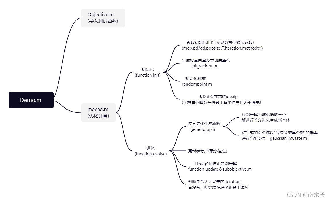
参数设置

• 种群规模(=权重向量个数=子问题个数)popsize：100；
• 邻居权重向量个数niche：20；
• 迭代次数iteration：250；
• 分解方法method：‘te’ or ‘ws’；
• 目标函数个数objDim：mop.od；
• 决策变量个数(决策空间维度)parDim：mop.pd；
• 参考点z：idealp。
  
  

代码中出现的几个主要结构体

objective.m
 p—>mop(也等价于randompoint.m中的prob)：两者结构相同是参数传递关系，存储MOP相关信息。

moead.m

1. function init：params(也等价于function pareto中的paramIn)：存储求解过程中的一些参数。
   
2. init_weight.m：p—>subp(也等价于moead.m中function pareto/init里的subproblems)：存储每个子问题的相关参数，具体内容见下图。
   
   说明：
   （1）optimal初始化为lnf，optpoint初始化为[ ]后好像就没有使用了;
   （2）curpoint还有一个estimation的字段（应该是存放两个评价指标值的），但是优化过程中没有进行评价，所以此处就不列出了。
3. randompoint.m：ind(等价于moead.m中function init里的inds)：用以存储当前点的所有信息，然后添加到subproblem的curpoint中。所以结构和上图中的curpoint相同。
   
   

Code

demo.m

 该函数为主函数。输入待优化函数信息及参数信息后即可成功完成代码运行。kno1函数决策空间的维度为2，其他函数的决策变量维度在原论文中可以找到。

     clc;clear;
 %% 导入测试函数
    disp('输入你想优化的函数');
    fun = input('kno1,zdt1—zdt4,zdt6,dtlz1/2：','s');
    dimension = input('number of decision variables：');
    mop = objective(fun, dimension);
    
%% 使用moead函数求解多目标最优解
    % 自定义种群规模，100，迭代次数，250，相邻种群数，20，方法，te
    pareto = moead(mop, 'popsize', 100, 'niche', 20, 'iteration', 1000, 'method', 'te');

    %pareto = moead( mop,'popsize', 100, 'niche', 20, 'iteration', 200, 'method', 'ws');

objective.m

 该函数根据输入的testname导入待优化的测试问题。测试问题和原论文保持一致，此处不再赘述。关于ZDT问题的一些解释可以参考进化计算（五）——NSGA-II论文阅读笔记（二）。【此处代码针对3-MOP问题进行的改动主要是增加了DTLZ1、DTLZ2两个测试问题，两者的决策变量维度都是10】

function mop = objective(testname, dimension)
%% 测试函数

%% main
    mop = struct('name', [], 'od', [], 'pd', [], 'domain', [], 'func', []);

    switch lower(testname)
    case 'kno1'
        mop = kno1(mop, dimension);
    case 'zdt1'
        mop = zdt1(mop, dimension);
    case 'zdt2' 
        mop = zdt2(mop, dimension);
    case 'zdt3' 
        mop = zdt3(mop, dimension);
    case 'zdt4' 
        mop = zdt4(mop, dimension);
    case 'zdt6' 
        mop = zdt6(mop, dimension); 
    case 'dtlz1' 
        mop = dtlz1(mop, dimension);
    case 'dtlz2' 
        mop = dtlz2(mop, dimension);         
    otherwise 
        error('Undefined test problem name');
    end 

end 

%% KNO1 function generator
% KNO1 问题的生成器

function p = kno1(p,dim)
    p.name = 'KNO1'; %名字
    p.od = 2; % 目标的维度
    p.pd = dim; % 参数的维度
    p.domain = [0 3; 0 3]; % 定义域
    p.func = @evaluate; % 评价函数

    % KNO1 evaluation function.
    % 定义评价函数
    function y = evaluate(x)
        y = zeros(2, 1);
        c = x(1) + x(2);
        f = 9 - (3 * sin(2.5 * c^0.5) + 3 * sin(4 * c) + 5 * sin(2 * c + 2));
        g = (pi / 2.0) * (x(1) - x(2) + 3.0) / 6.0;
        y(1) = 20 - (f * cos(g));
        y(2) = 20 - (f * sin(g));
    end 
end 

%% ZDT1 function generator

function p = zdt1(p, dim)
    p.name = 'ZDT1';
    p.pd = dim;
    p.od = 2;
    p.domain = [zeros(dim, 1) ones(dim, 1)];
    p.func = @evaluate;

    % ZDT1 evaluation function.
    function y = evaluate(x)
        y = zeros(2, 1);
        y(1) = x(1);
        su = sum(x) - x(1);
        g = 1 + 9 * su / (dim - 1);
        y(2) = g * (1 - sqrt(x(1) / g));
    end 
    load('ZDT1.txt');%导入正确的前端解
    plot(ZDT1(:,1),ZDT1(:,2),'k.');
    PP=ZDT1;
end 

%% ZDT2 function generator

function p = zdt2(p, dim)
    p.name = 'ZDT2';
    p.pd = dim; %决策变量的维度
    p.od = 2; %目标函数的个数
    p.domain = [zeros(dim, 1) ones(dim, 1)];
    p.func = @evaluate;

    % ZDT2 evaluation function.

    function y = evaluate(x)
        y = zeros(2, 1);
        y(1) = x(1);
        su = sum(x) - x(1);
        g = 1 + 9 * su / (dim - 1);
        y(2) = g * (1 - (x(1) / g)^2);
    end 
    load('ZDT2.txt');%导入正确的前端解
    plot(ZDT2(:,1),ZDT2(:,2),'k.');
    PP=ZDT2;
end 

%% ZDT3 function generator
function p = zdt3(p, dim)
    p.name = 'ZDT3';
    p.pd = dim;
    p.od = 2;
    p.domain = [zeros(dim, 1) ones(dim, 1)];
    p.func = @evaluate;

    % ZDT3 evaluation function.

    function y = evaluate(x)
        y = zeros(2, 1);
        y(1) = x(1);
        su = sum(x) - x(1);
        g = 1 + 9 * su / (dim - 1);
        y(2) = g * (1 - sqrt(x(1) / g) - x(1) * sin(10 * pi * x(1)) / g);
    end 
    load('ZDT3.txt');%导入正确的前端解
    plot(ZDT3(:,1),ZDT3(:,2),'k.');
    PP=ZDT3;
end 
%% ZDT4 function generator
function p = zdt4(p, dim)
    p.name = 'ZDT4';
    p.pd = dim;
    p.od = 2;
    x_min = [0,-5,-5,-5,-5,-5,-5,-5,-5,-5]';
    x_max=[1,5,5,5,5,5,5,5,5,5]';
    p.domain = [x_min x_max];
    p.func = @evaluate;

    % ZDT4 evaluation function.

    function y = evaluate(x)
        y = zeros(2, 1);
        y(1) = x(1);
        sum=0;
        for i=2:p.pd
            sum = sum+(x(i)^2-10*cos(4*pi*x(i)));
        end
        su = sum;
        g = 1 + 10 * (dim - 1) + su;
        y(2) = g * (1 - sqrt(x(1) / g));
    end 
    load('ZDT4.txt');%导入正确的前端解
    plot(ZDT4(:,1),ZDT4(:,2),'k.');
    PP=ZDT4;
end 
%% ZDT6 function generator
function p = zdt6(p, dim)
    p.name = 'ZDT6';
    p.pd = dim;
    p.od = 2;
    p.domain = [zeros(dim, 1) ones(dim, 1)];
    p.func = @evaluate;

    % ZDT6 evaluation function.

    function y = evaluate(x)
        y = zeros(2, 1);
        y(1)=1-(exp(-4*x(1)))*((sin(6*pi*x(1)))^6);
        su = sum(x) - x(1);
        g = 1 + 9 * ((su / (dim - 1))^0.25);
        y(2) = g * (1 - (y(1) / g)^2);
    end 
    load('ZDT6.txt');%导入正确的前端解
    plot(ZDT6(:,1),ZDT6(:,2),'k.');
    PP=ZDT6;
    
end 

%% DTLZ1 function generator
function p = dtlz1(p, dim)
    p.name = 'DTLZ1';
    p.pd = dim;
    p.od = 3;
    p.domain = [zeros(dim, 1) ones(dim, 1)];
    p.func = @evaluate;

    % DTLZ1 evaluation function.

    function y = evaluate(x)
        y = zeros(3, 1);
        sum = 0;
        for i=3:dim
          sum = sum+((x(i)-0.5)^2-cos(20*pi*(x(i)-0.5)));
        end       
        su = sum;
        g=100*(dim-2)+100*sum;
        y(1)=(1+g)*x(1)*x(2);
        y(2)=(1+g)*x(1)*(1-x(2));
        y(3)=(1+g)*(1-x(1));        
    end 
    load('DTLZ1.txt');%导入正确的前端解
    plot3(DTLZ1(:,1),DTLZ1(:,2),DTLZ1(:,3),'k.');
    PP=DTLZ1;
    
end

%% DTLZ2 function generator
function p = dtlz2(p, dim)
    p.name = 'DTLZ2';
    p.pd = dim;
    p.od = 3;
    p.domain = [zeros(dim, 1) ones(dim, 1)];
    p.func = @evaluate;

    % DTLZ2 evaluation function.

    function y = evaluate(x)
        y = zeros(3, 1);
        sum = 0;
        for i=3:dim
          sum = sum+(x(i))^2;
        end 
        g=sum;
        y(1)=(1+g)*cos(x(1)*pi*0.5)*cos(x(2)*pi*0.5);
        y(2)=(1+g)*cos(x(1)*pi*0.5)*sin(x(2)*pi*0.5);
        y(3)=(1+g)*sin(x(1)*pi*0.5);
    end 
    load('DTLZ2.txt');%导入正确的前端解
    plot3(DTLZ2(:,1),DTLZ2(:,2),DTLZ2(:,3),'g*');
    PP=DTLZ2;
    
end 

moead.m

 该函数为核心函数。主要由function pareto、function init、function evolve、function update以及function terminate组成。其中，pareto函数作为moead.m中的main函数，调用初始化函数init、进化函数evolve以及判断终止函数terminate完成MOEA/D算法的仿真。 进化函数evolve运行过程中调用update函数更新邻居解。各个函数的功能及其与原文算法框架的对应在代码中均有详细注释。【此处代码针对3-MOP问题进行的改动主要在结果显示部分】

function pareto = moead(mop, varargin)

    %MOEAD runs moea/d algorithms for the given mop.
    %   Detailed explanation goes here
    %   The mop must to be minimizing.
    %   The parameters of the algorithms can be set through varargin. including
    %   popsize: The subproblem's size.
    %   niche: the neighboursize, must less then the popsize.
    %   iteration: the total iteration of the moead algorithms before finish.
    %   method: the decomposition method, the value can be 'ws' or 'te'.
%% main

%------------------------------定义开始时间-------------------------------%
    starttime = clock;
  
%----------------------------定义一些全局变量-----------------------------%
    global params idealpoint objDim parDim itrCounter;
   
%-----------------------------定义随机生成器------------------------------%
   rand('state', 10); %锁定初始状态保证每次随机生成的状态相同,也可以不锁定
   % 对除zdt4外的函数，锁定与不锁定的区别不大。而对zdt4函数，代码每次会收敛
   % 到不同PF，所以不锁定的话每次得到的PF都不一样 
%---------------------------------初始化----------------------------------%
    paramIn = varargin;
    [objDim, parDim, idealpoint, params, subproblems] = init(mop, paramIn);

%--------------------------主循环：进化、更新-----------------------------%
    % 初始化循环编号
    itrCounter = 1;

    while ~terminate(itrCounter)
        tic;
        subproblems = evolve(subproblems, mop, params);
        fprintf('iteration %u finished, time used: %u\n', itrCounter, toc);
        itrCounter = itrCounter + 1;
    end 

%-------------------------------显示结果----------------------------------%
    pareto = [subproblems.curpoint];
    pp = [pareto.objective];
    [a,~]=size(pp);
    if(a==2)
    hold on;
    scatter(pp(1, :), pp(2, :));
    title(mop.name);
    fprintf('total time used %u\n', etime(clock, starttime));
    else 
    hold on;
    plot3(pp(1, :), pp(2, :),pp(3, :),'b.');
    title(mop.name);
    fprintf('total time used %u\n', etime(clock, starttime));
    end
end 

function [objDim, parDim, idealp, params, subproblems] = init(mop, propertyArgIn)
%% 初始化
    
    objDim = mop.od; % 获取目标的维度
    parDim = mop.pd; % 获取参数的维度
    idealp = ones(objDim, 1) * inf; %初始化参考点为lnf

%----------------------------固定参数的默认值-----------------------------%
    params.popsize = 100; params.niche = 30; params.iteration = 100;
    params.dmethod = 'te';
    params.F = 0.5;
    params.CR = 0.5;

%-----------------------将默认参数替换为自定义的参数----------------------%
    while length(propertyArgIn) >= 2
        prop = propertyArgIn{1}; 
        val = propertyArgIn{2}; 
        propertyArgIn = propertyArgIn(3:end);
        
        switch prop
        case 'popsize'
            % 种群规模
            params.popsize = val;
        case 'niche'
            %相邻种群规模
            params.niche = val;
        case 'iteration'
            % 迭代次数
            params.iteration = val;
        case 'method'
            % 方法
            params.dmethod = val;
        otherwise  
            warning('moea doesnot support the given parameters name');
        end 
        
    end 

%---------------初始化权重向量，将问题分解成多个单目标问题----------------%    
    subproblems = init_weights(params.popsize, params.niche, objDim);
    params.popsize = length(subproblems); 
    
%----------------------------初始化初始解---------------------------------%
    %每个子问题分配了一个初始化起点，初始化种群是所有初始化起点的集合
    % 种群个数就是子问题个数，也就是权重向量个数
    inds = randompoint(mop, params.popsize);
    %计算初始解的目标函数值V并存放在inds中(arrayfun：将函数应用于结构体数组的字段)
    [V, INDS] = arrayfun(@evaluate, repmat(mop, size(inds)), inds, 'UniformOutput', 0);
    [subproblems.curpoint] = INDS{:};
    
    
%---------------------------------初始化z---------------------------------%
    % 把最优点(所有问题中的最小目标函数值点)保存在idealp中作为参考点   
    v = cell2mat(V);
    idealp = min(idealp, min(v, [], 2));
    clear inds INDS V indcells;
end 

function subproblems = evolve(subproblems, mop, params)
%% MOEA/D优化
    global idealpoint;

    for i = 1:length(subproblems)
%-----------------生成算子：ind存放当前子问题新生成的y'-------------------%
        ind = genetic_op(subproblems, i, mop.domain, params);
       
%------------------------------更新z--------------------------------------%
 %比较y'的目标函数值与原始的参考点，如果满足y'的目标函数值更小，就更新参考点
        [obj, ind] = evaluate(mop, ind);
        idealpoint = min(idealpoint, obj);

%---------------------更新第i个子问题的邻居子问题的x----------------------%
        neighbourindex = subproblems(i).neighbour;
        subproblems(neighbourindex) = update(subproblems(neighbourindex), ind, idealpoint);
        clear ind obj neighbourindex;
    end 

end 

function subp = update(subp, ind, idealpoint)
%% 更新邻居解
    global params
    
%---------------------------求解y'的g^{te}值------------------------------%
    newobj = subobjective([subp.weight], ind.objective, idealpoint, params.dmethod);

%--------------------------求解当前x的g^{te}值----------------------------%
    oops = [subp.curpoint];
    oldobj = subobjective([subp.weight], [oops.objective], idealpoint, params.dmethod);

%---------------------------更新邻居子问题的解----------------------------%
    %对某个邻居子问题，如果y'的g^{te}值<当前x的g^{te}值
    %那么就更新该邻居子问题的解，即令y'=当前x
    C = newobj < oldobj;%小于为1，不小于为0 
    [subp(C).curpoint] = deal(ind);
    clear C newobj oops oldobj;
end 

function y = terminate(itrcounter)
%% 判断停止迭代条件

    global params;
    y = itrcounter > params.iteration;
end 

Function init调用的外部函数

init_weights.m

 该函数的主要目的是初始化权重向量生成子问题，并找到每个子问题的20个邻居。对二维目标空间，代码中定义第$i$个子问题的权重向量为
$$\begin{gathered} weigh{t}_1=\frac{i}{popsize} \\ weigh{t}_2=\frac{popsize-i}{popsize} \\ whichsatisfies\text{ :}\sum _{i=1}^{m}weigh{t}_i=1 \end{gathered}$$
 此处与论文中使用的权重向量初始化的方法不太一样，但是也达到了论文中要求的权重向量的均匀分布。
 求解邻居向量时，分别计算两两向量之间的欧式距离$\sqrt{A^2-B^2}$构成距离矩阵$distanceMatrix$。排序后将邻居索引值存放在subp结构体的neighbour中。
 【此处为3-MOP代码改动的核心部分，主要是增加了随机生成均匀分布的三目标函数权重向量。代码中使用lhsdesign函数进行随机抽样，然后使用归一化方法约束权重向量满足${\sum }_{j=1}^3{w}_j=1$的条件。个人认为3-MOP优化效果不好可能是因为此处对于子问题生成的方法不合适的问题。如果想要获得更好的三目标优化结果，可以考虑从此处进行改进。】

function subp = init_weights(popsize, niche, objDim)
%% 初始化权重向量并找到每个向量的20个邻居向量
%% 初始化权值向量
    subp = [];
%--------------------------------二维目标空间-----------------------------%       
    if objDim == 2
      %循环所有种群规模
       for i = 0:popsize
        % 每个子问题都有
        p = struct('weight', [], 'neighbour', [], 'optimal', Inf, 'optpoint', [], 'curpoint', []);
        % 平均划分，定义每个权值向量，然后把定义好的所有向量装进subp
        weight = zeros(2, 1);
        weight(1) = i / popsize;
        weight(2) = (popsize - i) / popsize;
        p.weight = weight;
        subp = [subp p];
       end 
%--------------------------------三维目标空间-----------------------------%    
    elseif objDim == 3
        for i = 0:popsize
    %lhsdesign:lhsdesign函数是基本的拉丁超立方抽样的函数，总体的抽样结果服从均匀分布，
    %返回一个 n × p 的矩阵，每一列的元素是随机排列的。n为样本空间的分层数，p为样本维度数
            p=struct('weight', [], 'neighbour', [], 'optimal', Inf, 'optpoint', [], 'curpoint', []);
            weight=lhsdesign(1,3,'criterion', 'maximin', 'iterations', 1000);
            W=sum(weight);
            weight=weight./W;
            p.weight=weight';
            subp =[subp p];
        end
     end 

%% 求解邻居向量

    % 根据欧式距离求解邻居向量B(i)
    leng = length(subp);
    distanceMatrix = zeros(leng, leng); % 初始化距离矩阵

    % 计算每两个点间的距离
    for i = 1:leng
        for j = i + 1:leng

            A = subp(i).weight; B = subp(j).weight;
            distanceMatrix(i, j)= 0;
            for n=1:objDim
               distanceMatrix(i, j)=(A(n)-B(n))^2+distanceMatrix(i, j);
            end
            distanceMatrix(i, j)=sqrt(distanceMatrix(i, j));
            distanceMatrix(j, i) = distanceMatrix(i, j);
            
        end 
        
        %对第i个权重向量与其他权重向量之间的距离以及其他权重向量的索引进行排序
        %分别存放到s与sindex中
        [s, sindex] = sort(distanceMatrix(i, :));
        
        %将第i个子问题的邻居向量索引填入其结构体的对应元素neighbour中
        subp(i).neighbour = sindex(1:niche)';
    end 

end 

randompoint.m

 该函数主要用于在决策空间范围内生成所有子问题的初始解。在前边的NSGA-Ⅱ代码以及简单的遗传算法求解单目标问题代码中都有类似的步骤，只不过该代码中采用了结构体的形式存放初始解，处理过程中多了许多与结构体相关的步骤。基本思想还是容易理解的:
$$\begin{gathered} △=upperbound-lowerbound \\ solution=random\times △+lowerbound \\ s.t.random\in (0,1) \end{gathered}$$
 其他的操作在代码中均有详细注释。

function ind = randompoint(prob, n)
%% 在定义域范围内随机采样生成初始解\vec{x}
   %n = popsize
   
    if (nargin == 1)
        n = 1;
    end 

    % 在决策空间范围内随机采样生成初始解
    randarray = rand(prob.pd, n);
    lowend = prob.domain(:, 1); %决策变量下界
    span = prob.domain(:, 2) - lowend; %决策变量上下界之间的最大差值
    a = span(:, ones(1, n)); %30×1—>30×101
    b = lowend(:, ones(1, n)); %30×1—>30×101
    point = randarray .* a + b;  %生成的解要在决策空间范围内

    % 然后把生成的随机数变成变成元孢便于存放在当前解的结构体ind中
    cellpoints = num2cell(point, 1);

    % 把生成的元孢装进ind中的parameter里
    indiv = struct('parameter', [], 'objective', [], 'estimation', []);
    ind = repmat(indiv, 1, n);
    [ind.parameter] = cellpoints{:};
    
     estimation = struct('obj', NaN, 'std', NaN);
     [ind.estimation] = deal(repmat(estimation, prob.od, 1));
end 

evaluate.m

 该函数主要用于计算解的目标函数值。源代码中对$x$是结构体和不是结构体分两种情况进行计算，实际运行中输入的解始终是结构体的形式，所以只要理解该函数是计算当前解的目标函数值即可。moead.m中的arrayfun函数作用是将函数应用于结构体数组的字段。

%EVALUATE function evaluate an individual structure of a vector point with
%the given multiobjective problem.

%   Detailed explanation goes here
%   prob: is the multiobjective problem.
%   x: is a vector point, or a individual structure.
%   v: is the result objectives evaluated by the mop.
%   x: if x is a individual structure, then x's objective field is modified
%   with the evaluated value and pass back.

%   TODO, need to refine it to operate on a vector of points.
    if isstruct(x)
        v = prob.func(x.parameter);
        x.objective=v;
    else
        v = prob.func(x);
    end

Function evolve调用的外部函数

genetic_op.m

 该步主要是引用了差分进化中的变异思想。代码中对当前子问题使用它的三个邻居子问题进行差分进化操作生成后代。主要操作为：在第$g$次迭代时，使用三个邻居子问题的当前解差分计算生成后代$$newpoint(g)=selectpoin{t}_1(g)+F\cdot (selectpoin{t}_2(g)-selectpoin{t}_3(g))$$
 其中，缩放因子$F=0.5$。当前优化子问题的当前解中每个维度的取值都以$CR=0.5$的概率进化成$newpoint$对应维度中的值。完成进化后还应保证子代位于决策变量空间(定义域)范围内，对于超出范围的值直接做截断处理(e.g.定义域范围为[0,1]，那么小于0的维度值置为0，大于1的维度值置为1)，相当于原始论文中提到的$repair$修复$y$为$y^{\prime }$。完成上述操作后，再通过一次$gaussianmutate$生成当前子问题的最终子代。

function ind = genetic_op(subproblems, index, domain, params)
%% 使用当前的种群进行差分进化
    %GENETICOP function implemented the DE operation to generate a new
    %individual from a subproblems and its neighbours.

    %   subproblems: 所有的子问题
    %   index: 当前正在优化的子问题的编号
    %   domain: 多目标优化问题解的定义域
    %   ind: 个体结构体
    
%% 提取出邻居矩阵
    neighbourindex = subproblems(index).neighbour;
    
%% 从所有邻居中进行随机抽取三个不同的子问题
    nsize = length(neighbourindex);
    si = ones(1, 3) * index;

    si(1) = neighbourindex(ceil(rand * nsize));%ceil

    while si(1) == index  %确保寻找的邻居子问题索引不是当前正在优化的子问题索引
        si(1) = neighbourindex(ceil(rand * nsize));
    end 

    si(2) = neighbourindex(ceil(rand * nsize));

    while si(2) == index || si(2) == si(1) %确保寻找的所有邻居子问题索引不同
        si(2) = neighbourindex(ceil(rand * nsize));
    end 

    si(3) = neighbourindex(ceil(rand * nsize));

    while si(3) == index || si(3) == si(2) || si(3) == si(1)
        si(3) = neighbourindex(ceil(rand * nsize));
    end 
    
%%  选择变异生成新x  
    points = [subproblems(si).curpoint]; 
    selectpoints = [points.parameter];   %选定三个邻居子问题的当前解

    oldpoint = subproblems(index).curpoint.parameter; %原始解为当前子问题的当前解
    parDim = size(domain, 1); 
    
    jrandom = ceil(rand * parDim);  %四舍五入生成一个小于等于parDim的整数

    randomarray = rand(parDim, 1); %随机生成一列（0，1）范围内的向量
    
    %randomarray中小于CR(0.5)的索引处为deselect为1，其他点为0
    deselect = randomarray < params.CR;
    
    %保证原始解中第jrandom个维度元素值不变，所以设置deselect_jrandom=1
    deselect(jrandom) = true;%x_jrandom=1
    
    %使用三个邻居子问题的当前解生成新解，此处F=0.5
    newpoint = selectpoints(:, 1) + params.F * (selectpoints(:, 2) - selectpoints(:, 3));
    
    %若deselect中某一维度值为0，则当前解的该维度值不变，为1变异更新为newpoint中的值
    newpoint(~deselect) = oldpoint(~deselect); 

%% 规范新找到的点在定义域范围内
    newpoint = max(newpoint, domain(:, 1));
    newpoint = min(newpoint, domain(:, 2));
    ind = struct('parameter', newpoint, 'objective', [], 'estimation', []);
    
%% 对新找到的点进行高斯变异生成最终的子代
    ind = gaussian_mutate(ind, 1 / parDim, domain);
    
end 

gaussian_mutate.m

 该函数主要用于对差分进化生成的后代进行变异。首先由高斯变异算子生成变异后子代，然后个体向量中的每个元素以$“1/parDim”$的概率最终确定是否进行变异。变异结果很明显的优化了ZDT2、ZDT6、ZDT4这三个函数得到的PF。如果不进行gaussian_mutate，算法在这三个函数上的收敛性和分布性很差，得到的解质量不高。进行gaussian_mutate后，对这三个函数的优化可以明显的收敛到真实PF上。代码如下：

function ind = gaussian_mutate( ind, prob, domain)
%% 高斯变异，变异概率为"1/决策空间维度"

   x = ind.parameter;
   parDim = length(x);
   lowend  = domain(:,1);
   highend =domain(:,2);
   sigma = (highend-lowend)./20; %标准差
   
%r = normrnd(mu,sigma) generates a random number from the normal distribu-
%   tion with mean parameter mu and standard deviation parameter sigma.

   newparam = min(max(normrnd(x, sigma), lowend), highend);
   C = rand(parDim, 1)<prob; %小于为1，不小于为0
   x(C) = newparam(C);
   
   ind.parameter = x;
end

 简单介绍一下高斯变异：高斯变异（Gaussian Mutation）操作是指进行变异操作时，用符合均值为$\mu$标准差为$\sigma$的正态分布的一个随机数来替代原有的基因值。决策空间定义在$(a,b)$上。令$x\in (a,b)$，高斯生成算子将$x$变异为$M_G$:
$$M_G=min(max(N(x,\sigma ),a),b)$$
 高斯变异中的$\sigma$取值依赖于定义域长度，通常取$\sigma =(b-a)/10$，上述代码中取$\sigma =(b-a)/20$。对$\sigma$的选取还有许多可优化的方法，如随时间(不同迭代次数)减小、选取两个不同的变异算子(一个是较大的$\sigma$值，一个是较小的$\sigma$值)等等。更多内容可以参考这个网站。
 由正态分布的特性可知，高斯变异也是重点搜索原个体附近的某个局部区域。高斯变异主要在于依托一个高斯分布对个体向量中的每一个元素增加一个随机值从而创建一个新的后代。

 高斯变异的局部搜索能力较好，但是引导个体跳出局部较优解的能力较弱，不利于全局收敛。

Func update调用的外部函数

subobjective.m

 该目标函数主要是用于更新邻居解步骤求解$g^{te}$值或者$g^{ws}$值。由于代码中会对生成的单个新解以及所有子问题的当前解分别求解$g^{te}$值或$g^{ws}$值，所以源代码中分情况进行了编写。理解代码时只要了解该部分代码是为了在更新邻居解时求解$g^{te}$值或$g^{ws}$值使用即可。
 【此处虽然没有进行针对3-MOP问题的改动，但是原文中也提到了如果能够使用更好的分解方法就可以使得到的近似PF收敛性和分布性大大提高，因此也可以考虑从该部分着手进行优化：如使用原文中的PBI（带约束的边界聚合方法）完成优化收敛步骤。】

function obj = subobjective(weight, ind, idealpoint, method)
%% 求解g^{te}或者g^{ws}值
%   应用切比雪夫和加权和两种方法
%   weight: 所有子问题的权重向量 (列向量).
%   ind: 新解的目标函数值 (列向量)/所有子问题的当前解的目标函数值（列向量集）.
%   idealpoint: 当前的参考点的目标函数值.
%   method: 选择的分解方法，默认是切比雪夫“te”
%   nargin: 函数输入参数个数
%   
%   weight和ind也可以是矩阵，有如下两种情况：
%  （1）当weight是矩阵时，它就被看作按列排列的权重集。在这种情况下，如果ind
%   是一个列向量(输入新解的目标函数值)，subobjective就使用每一个权重和ind计
%   算；
%  （2）如果 ind 也是一个与weight大小相同的矩阵(输入所有子问题当前解的目标
%   函数值)，那么子目标将在列到列中计算，权重的每一列都针对 ind 的相应列进
%   行计算。
%
%   在上述两种情况中，subobjective都会返回一个行向量。

%% main
    if (nargin==2) %通过输入的参数值判断调用的分解方法
            obj = ws(weight, ind);
        elseif (nargin==3)
            obj = te(weight, ind, idealpoint);
    else           %通过输入的method确定调用的分解方法
        if strcmp(method, 'ws') 
            obj=ws(weight, ind);
        elseif strcmp(method, 'te')
            obj=te(weight,  ind, idealpoint);
        else
            obj= te(weight, ind, idealpoint);
        end
    end
end

%% 加权和方法
function obj = ws(weight, ind)
    if size(ind, 2) == 1    %只有一个目标函数向量（求解新解的g^{te}值）
       obj = (weight'*ind)'; 
    else
       obj = sum(weight.*ind); %有s个目标函数向量（求解所有子问题的当前解的g^{te}值）
    end
end

%% 切比雪夫方法
function obj = te(weight, ind, idealpoint)
    s = size(weight, 2); %子问题个数（权重向量个数）
    indsize = size(ind,2); %目标函数个数
    
    weight((weight == 0))=0.00001;
    
    if indsize==s 
        part2 = abs(ind-idealpoint(:,ones(1, indsize)));
        obj = max(weight.*part2);
    elseif indsize ==1
        part2 = abs(ind-idealpoint);
        obj = max(weight.*part2(:,ones(1, s)));   
    else
        error('individual size must be same as weight size, or equals 1');
    end
end

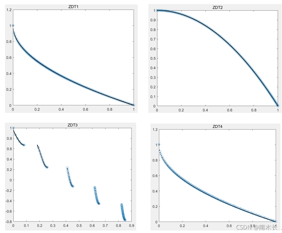
Result

切比雪夫分解

测试问题	耗时
zdt1	7.906s
zdt2	7.829s
zdt3	7.731s
zdt4	7.802s
zdt6	7.447s
kno1	7.801s

优化结果：

加权和分解

 使用加权和分解得到的结果分布性较差，收敛性相较切比雪夫分解方法仍有一定的差距，但是和之前的NSGA-Ⅱ算法相比收敛性还不错。优化耗时和切比雪夫分解方法持平，但是会出现存在较大偏差的点。下面给出部分典型结果：

一点点思考

 MOEA/D原文详解中花了很多的篇幅重点介绍三种不同的分解方法：加权和、切比雪夫、边界聚合以及作者提出的PBI。但是在实际算法执行时，三种分解算法并不是用于将多目标问题分解成不同的子问题(即完成所谓的“分解”操作：生成不同的权重向量)，而是在优化过程中用于更新邻居解，从而使所求解逐代向真实PF收敛。总结来说，三种分解方法的目标是解决分解后如何对众多子问题进行优化的问题，而不是解决如何将多目标问题分解的多个单目标子问题的问题。

参考文献及链接

[1]Qingfu Zhang, Hui Li.MOEA/D: A Multiobjective Evolutionary Algorithm Based on Decomposition[J].IEEE ；
[2]差分进化算法；
[3]高斯变异1；
[4]高斯变异2；

其他推荐的代码

 这个代码和原论文中的算法过程完全契合，但是二目标MOP优化结果会略逊于上文中代码的优化结果，且算法运行时间没有得到特别大的改善。但是这个代码对于读者进行原论文算法流程的理解以及进行与NSGA-Ⅱ算法优化结果的对比这两方面十分友好，所以在这边也推荐一下:
多目标优化算法(二)MOEAD（附带NSGA2）的文档和代码（MATLAB）。