
机器学习——特征工程——交互特征(多项式特征)
两个特征的乘积可以组成一对简单的交互特征,这种相乘关系可以用逻辑操作符AND来类比,它可以表示出由一对条件形成的结果:“该购买行为来自于邮政编码为98121的地区”AND“用户年龄在18和35岁之间”。这种特征在基于决策树的模型中极其常见,在广义线性模型中也经常使用。简单线性模型使用独立输入特征, , …, 的线性组合来预测结果变量:。很容易对线性模型进行扩展,使之包含输入特征的两两组合,如下所示
一、交互特征定义
两个特征的乘积可以组成一对简单的交互特征,这种相乘关系可以用逻辑操作符AND来类比,它可以表示出由一对条件形成的结果:“该购买行为来自于邮政编码为98121的地区”AND“用户年龄在18和35岁之间”。这种特征在基于决策树的模型中极其常见,在广义线性模型中也经常使用。
简单线性模型使用独立输入特征,
, …,
的线性组合来预测结果变量
:
。
很容易对线性模型进行扩展,使之包含输入特征的两两组合,如下:。
这样,就可以捕获特征之间的交互作用,因此这些特征对就称为交互特征。如果和
是二值特征,那么它们的积
就是逻辑函数
AND
。如果我们的问题是基于客户档案信息来预测客户偏好,那么在这个例子中,除了根据用户的年龄或地点这些单独特征来进行预测,还可以使用交互特征来根据用户位于某个年龄段并且位于某个特定地点来进行预测。
二、sklearn的PolynomialFeatures的用法
使用 sklearn.preprocessing.PolynomialFeatures 这个类可以进行特征的构造,构造的方式就是特征与特征相乘(自己与自己,自己与其他人),这种方式叫做使用多项式的方式。例如:有、
两个特征,那么它的 2 次多项式的次数为 [
]。
PolynomialFeatures 这个类有 3 个参数:
- degree:控制多项式的次数;
- interaction_only:默认为 False,如果指定为 True,那么就不会有特征自己和自己结合的项,组合的特征中没有
和
;
- include_bias:默认为 True 。如果为 True 的话,那么结果中就会有 0 次幂项,即全为 1 这一列。
1、案例一:多项式特征构造过程
1.1、建立数据
from sklearn.preprocessing import PolynomialFeatures
import numpy as np
X=np.arange(6).reshape(3,2)
X
输出:
array([[0, 1],
       [2, 3],
       [4, 5]])
1.2、设置多项式阶数为2,其他默认。
poly1=PolynomialFeatures(degree=2)
res1=poly1.fit_transform(X)
res1
输出:
array([[ 1.,  0.,  1.,  0.,  0.,  1.],
       [ 1.,  2.,  3.,  4.,  6.,  9.],
       [ 1.,  4.,  5., 16., 20., 25.]])
interaction_only,默认为 False,既组合的特征中有和
;include_bias,默认为 True,那么结果中就会有
,即全为 1 这一列。如果interaction_only设置为True,include_bias设置为False,则会变成如下:
poly2=PolynomialFeatures(interaction_only=True,include_bias=False)
res2=poly2.fit_transform(X)
res2
输出:
array([[ 0.,  1.,  0.],
       [ 2.,  3.,  6.],
[ 4., 5., 20.]])既少了这三列。
1.3、PolynomialFeatures可返回的参数
输出转换之后的特征名称:
poly1.get_feature_names()输出:
['1', 'x0', 'x1', 'x0^2', 'x0 x1', 'x1^2']我们可以输出数据的转换次数(幂):
#输出6个特征,来自原来的2个特征的幂(转变过程)
poly1.powers_
输出:
array([[0, 0],
       [1, 0],
       [0, 1],
       [2, 0],
       [1, 1],
       [0, 2]], dtype=int64)
其中:
[0,0]表示新特征由原始特征这样组成:,其实就是1这一列;
[1,0]表示新特征由原始特征这样组成:,其实就是
这一列;
[0,1]表示新特征由原始特征这样组成:,其实就是
这一列;
[2,0]表示新特征由原始特征这样组成:,其实就是
这一列;
[1,1]表示新特征由原始特征这样组成:,其实就是
这一列;
[0,2]表示新特征由原始特征这样组成:,其实就是
这一列;
同样,我们可以输出转换前后的特征个数:
#输出原始特征个数
poly1.n_input_features_

#输出多项式转换之后的特征个数
poly1.n_output_features_
输出:
2

6
2、案例二:多项式特征应用于回归模型
2.1、建立数据
from sklearn.linear_model import LinearRegression
from sklearn.tree import DecisionTreeRegressor
from sklearn.preprocessing import PolynomialFeatures
import mglearn
import numpy as np
import matplotlib.pyplot as plt

#建立数据
X, y = mglearn.datasets.make_wave(n_samples=100) #100个样本点
X.shape

y.shape

#辅助数据,用于绘制回归曲线
line = np.linspace(-3, 3, 1000, endpoint=False).reshape(-1, 1)
line.shape
输出:
(100, 1)

(100,)

(1000, 1)
2.2、构造多项式特征
#包含到x^10的多项式
#默认的include_bias=True添加恒等于1的常数特征
poly = PolynomialFeatures(degree=10, include_bias=False)
poly.fit(X)
X_poly = poly.transform(X)
X_poly.shape

poly.get_feature_names()

X_poly[:5]

X[:5]
输出:
(100, 10)

['x0', 'x0^2', 'x0^3', 'x0^4', 'x0^5', 'x0^6', 'x0^7', 'x0^8', 'x0^9', 'x0^10']

array([[-7.52759287e-01,  5.66646544e-01, -4.26548448e-01,
         3.21088306e-01, -2.41702204e-01,  1.81943579e-01,
        -1.36959719e-01,  1.03097700e-01, -7.76077513e-02,
         5.84199555e-02],
       [ 2.70428584e+00,  7.31316190e+00,  1.97768801e+01,
         5.34823369e+01,  1.44631526e+02,  3.91124988e+02,
         1.05771377e+03,  2.86036036e+03,  7.73523202e+03,
         2.09182784e+04],
       [ 1.39196365e+00,  1.93756281e+00,  2.69701700e+00,
         3.75414962e+00,  5.22563982e+00,  7.27390068e+00,
         1.01250053e+01,  1.40936394e+01,  1.96178338e+01,
         2.73073115e+01],
       [ 5.91950905e-01,  3.50405874e-01,  2.07423074e-01,
         1.22784277e-01,  7.26822637e-02,  4.30243318e-02,
         2.54682921e-02,  1.50759786e-02,  8.92423917e-03,
         5.28271146e-03],
       [-2.06388816e+00,  4.25963433e+00, -8.79140884e+00,
         1.81444846e+01, -3.74481869e+01,  7.72888694e+01,
        -1.59515582e+02,  3.29222321e+02, -6.79478050e+02,
         1.40236670e+03]])

array([[-0.75275929],
       [ 2.70428584],
       [ 1.39196365],
       [ 0.59195091],
[-2.06388816]]) 从上面我们可以得出,多项式特征的构成过程为,从1列变成了10列。
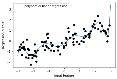
2.3、回归模型训练及可视化
将多项式特征与回归模型一起使用,可以得到经典的多项式回归。
reg = LinearRegression().fit(X_poly, y)

line_poly = poly.transform(line)
plt.plot(line, reg.predict(line_poly), label='polynomial linear regression')
plt.plot(X[:, 0], y, 'o', c='k')
plt.ylabel("Regression output")
plt.xlabel("Input feature")
plt.legend(loc="best")
输出:
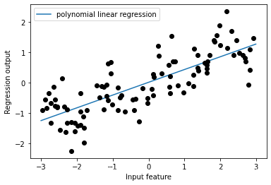
原始没有进行转换的数据,结合回归模型,得到的是简单的线性回归模型。
reg = LinearRegression().fit(X, y)

line_poly = poly.transform(line)
plt.plot(line, reg.predict(line), label='linear regression')
plt.plot(X[:, 0], y, 'o', c='k')
plt.ylabel("Regression output")
plt.xlabel("Input feature")
plt.legend(loc="best")
输出:
作为对比,下面用较复杂的模型——核SVM模型来学习原始数据,原数据没有做任何变换。
from sklearn.svm import SVR

for gamma in [1, 10]:
    svr = SVR(gamma=gamma).fit(X, y)
    plt.plot(line, svr.predict(line), label='SVR gamma={}'.format(gamma))

plt.plot(X[:, 0], y, 'o', c='k')
plt.ylabel("Regression output")
plt.xlabel("Input feature")
plt.legend(loc="best")
输出:
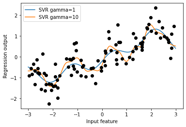
以上我们可以得到:使用更为复杂的模型(如核SVM),且不需要进行显式地特征变换,我们也能够学习到一个与多项式回归(简单回归+多项式特征转换)复杂度类似的预测结果。
3、案例三:NFL原则讨论
3.1、采用波士顿房价数据集,利用MinMaxScaler将其放缩到0-1之间
from sklearn.datasets import load_boston
from sklearn.model_selection import train_test_split
from sklearn.preprocessing import MinMaxScaler

boston = load_boston()
X_train, X_test, y_train, y_test = train_test_split(
    boston.data, boston.target, random_state=0)

# MinMaxScaler
scaler = MinMaxScaler()
X_train_scaled = scaler.fit_transform(X_train)
X_test_scaled = scaler.transform(X_test)
3.2、提取多项式特征和交互特征
poly = PolynomialFeatures(degree=2).fit(X_train_scaled)
X_train_poly = poly.transform(X_train_scaled)
X_test_poly = poly.transform(X_test_scaled)
print("X_train.shape: {}".format(X_train.shape))
print("X_train_poly.shape: {}".format(X_train_poly.shape))
print("Polynomial feature names:\n{}".format(poly.get_feature_names()))
输出:
X_train.shape: (379, 13)

X_train_poly.shape: (379, 105)

Polynomial feature names:
['1', 'x0', 'x1', 'x2', 'x3', 'x4', 'x5', 'x6', 'x7', 'x8', 'x9', 'x10', 'x11', 'x12', 'x0^2', 'x0 x1', 'x0 x2', 'x0 x3', 'x0 x4', 'x0 x5', 'x0 x6', 'x0 x7', 'x0 x8', 'x0 x9', 'x0 x10', 'x0 x11', 'x0 x12', 'x1^2', 'x1 x2', 'x1 x3', 'x1 x4', 'x1 x5', 'x1 x6', 'x1 x7', 'x1 x8', 'x1 x9', 'x1 x10', 'x1 x11', 'x1 x12', 'x2^2', 'x2 x3', 'x2 x4', 'x2 x5', 'x2 x6', 'x2 x7', 'x2 x8', 'x2 x9', 'x2 x10', 'x2 x11', 'x2 x12', 'x3^2', 'x3 x4', 'x3 x5', 'x3 x6', 'x3 x7', 'x3 x8', 'x3 x9', 'x3 x10', 'x3 x11', 'x3 x12', 'x4^2', 'x4 x5', 'x4 x6', 'x4 x7', 'x4 x8', 'x4 x9', 'x4 x10', 'x4 x11', 'x4 x12', 'x5^2', 'x5 x6', 'x5 x7', 'x5 x8', 'x5 x9', 'x5 x10', 'x5 x11', 'x5 x12', 'x6^2', 'x6 x7', 'x6 x8', 'x6 x9', 'x6 x10', 'x6 x11', 'x6 x12', 'x7^2', 'x7 x8', 'x7 x9', 'x7 x10', 'x7 x11', 'x7 x12', 'x8^2', 'x8 x9', 'x8 x10', 'x8 x11', 'x8 x12', 'x9^2', 'x9 x10', 'x9 x11', 'x9 x12', 'x10^2', 'x10 x11', 'x10 x12', 'x11^2', 'x11 x12', 'x12^2']
3.3、对Ridge(岭回归)在有交互特征地数据集和没有交互特征地数据上地性能进行对比
from sklearn.linear_model import Ridge
ridge = Ridge().fit(X_train_scaled, y_train)
print("Score without interactions: {:.3f}".format(
    ridge.score(X_test_scaled, y_test)))
ridge = Ridge().fit(X_train_poly, y_train)
print("Score with interactions: {:.3f}".format(
    ridge.score(X_test_poly, y_test)))
输出:
Score without interactions: 0.621
Score with interactions: 0.753
显然,在使用Ridge(岭回归)时,交互特征和多项式特征对性能有很大地提升。但如果使用更复杂地模型(比如随机森林),情况可能会稍有不同。如下:
from sklearn.ensemble import RandomForestRegressor
rf = RandomForestRegressor(n_estimators=100).fit(X_train_scaled, y_train)
print("Score without interactions: {:.3f}".format(
    rf.score(X_test_scaled, y_test)))
rf = RandomForestRegressor(n_estimators=100).fit(X_train_poly, y_train)
print("Score with interactions: {:.3f}".format(rf.score(X_test_poly, y_test)))
输出:
Score without interactions: 0.807
Score with interactions: 0.777
可以看出,即使没有额外的特征, 随机森林的性能也要优于Ridge(岭回归)。添加交互项特征和多项式特征实际上会略微降低其性能。关于此方面问题,大家想深入了解的话,可见《 NFL定理》。
更多推荐


 12
12 0
0- 0


 已为社区贡献2条内容

所有评论(0)