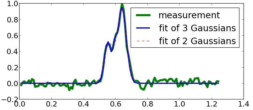
I've been looking for a way to do multiple Gaussian fitting to my data. Most of the examples I've found so far use a normal distribution to make random numbers. But I am interested in looking at the plot of my data and checking if there are 1-3 peaks.
I can do this for one peak, but I don't know how to do it for more.
For example, I have this data: http://www.filedropper.com/data_11
I have tried using lmfit, and of course scipy, but with no nice results.
Thanks for any help!
Simply make parameterized model functions of the sum of single Gaussians. Choose a good value for your initial guess (this is a really critical step) and then have scipy.optimize tweak those numbers a bit.
Here's how you might do it:
import numpy as np
import matplotlib.pyplot as plt
from scipy import optimize

data = np.genfromtxt('data.txt')
def gaussian(x, height, center, width, offset):
    return height*np.exp(-(x - center)**2/(2*width**2)) + offset
def three_gaussians(x, h1, c1, w1, h2, c2, w2, h3, c3, w3, offset):
    return (gaussian(x, h1, c1, w1, offset=0) +
        gaussian(x, h2, c2, w2, offset=0) +
        gaussian(x, h3, c3, w3, offset=0) + offset)

def two_gaussians(x, h1, c1, w1, h2, c2, w2, offset):
    return three_gaussians(x, h1, c1, w1, h2, c2, w2, 0,0,1, offset)

errfunc3 = lambda p, x, y: (three_gaussians(x, *p) - y)**2
errfunc2 = lambda p, x, y: (two_gaussians(x, *p) - y)**2

guess3 = [0.49, 0.55, 0.01, 0.6, 0.61, 0.01, 1, 0.64, 0.01, 0]  # I guess there are 3 peaks, 2 are clear, but between them there seems to be another one, based on the change in slope smoothness there
guess2 = [0.49, 0.55, 0.01, 1, 0.64, 0.01, 0]  # I removed the peak I'm not too sure about
optim3, success = optimize.leastsq(errfunc3, guess3[:], args=(data[:,0], data[:,1]))
optim2, success = optimize.leastsq(errfunc2, guess2[:], args=(data[:,0], data[:,1]))
optim3

plt.plot(data[:,0], data[:,1], lw=5, c='g', label='measurement')
plt.plot(data[:,0], three_gaussians(data[:,0], *optim3),
    lw=3, c='b', label='fit of 3 Gaussians')
plt.plot(data[:,0], two_gaussians(data[:,0], *optim2),
    lw=1, c='r', ls='--', label='fit of 2 Gaussians')
plt.legend(loc='best')
plt.savefig('result.png')

As you can see, there is almost no difference between these two fits (visually). So you can't know for sure if there were 3 Gaussians present in the source or only 2. However, if you had to make a guess, then check for the smallest residual:
err3 = np.sqrt(errfunc3(optim3, data[:,0], data[:,1])).sum()
err2 = np.sqrt(errfunc2(optim2, data[:,0], data[:,1])).sum()
print('Residual error when fitting 3 Gaussians: {}\n'
    'Residual error when fitting 2 Gaussians: {}'.format(err3, err2))
# Residual error when fitting 3 Gaussians: 3.52000910965
# Residual error when fitting 2 Gaussians: 3.82054499044
In this case, 3 Gaussians gives a better result, but I also made my initial guess fairly accurate.


 已为社区贡献126442条内容

所有评论(0)