
【端侧部署系列】EfficientVit_seg部署至全志开发板
简介
EfficientVit开源项目所在的github仓库地址:https://github.com/mit-han-lab/efficientvit
官方基于Cityscapes(城市街景),和ADE20K(室内外场景)两种数据集分别进行了模型训练,并提供了模型权重,本文以Cityscapes图像分割为例进行测试。
Cityscapes数据集https://www.cityscapes-dataset.com/
EfficientViT针对不同的性能要求,提供了多个版本的efficientvit,L(大模型)和B(轻量)。
本文使用EfficientViT-B1测试,官方权重下载链接如下:
| Model | Resolution | Cityscapes mIoU | Params | MACs | Jetson Nano (bs1) | Jetson Orin (bs1) | Checkpoint |
|---|---|---|---|---|---|---|---|
| EfficientViT-B0 | 1024x2048 | 75.653 | 0.7M | 4.4G | 275ms | 9.9ms | link |
| EfficientViT-B1 | 1024x2048 | 80.547 | 4.8M | 25G | 819ms | 24.3ms | link |
| EfficientViT-B2 | 1024x2048 | 82.073 | 15M | 74G | 1676ms | 46.5ms | link |
| EfficientViT-B3 | 1024x2048 | 83.016 | 40M | 179G | 3192ms | 81.8ms | link |
pt模型推理
在开源项目efficientvit-master文件中,将下载的权重放置assets/checkpoints/efficientvit_seg/中,执行下列代码进行测试,若没有cuda,删除demo_efficientvit_seg_model.py中的.cuda()操作,禁止调用cuda。
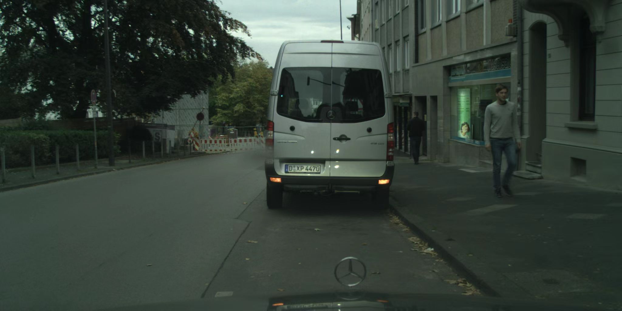
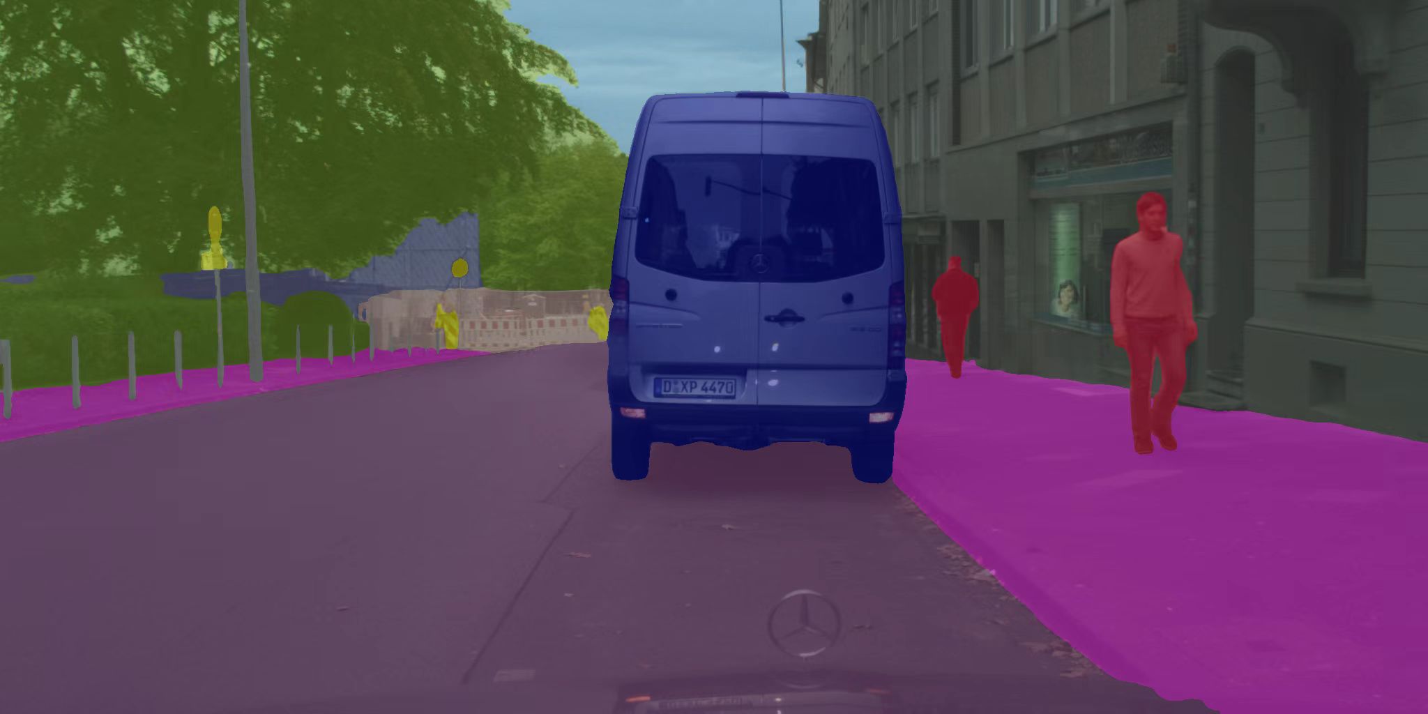
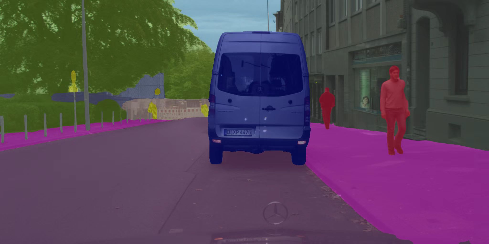
python applications/efficientvit_seg/demo_efficientvit_seg_model.py --image_path assets/fig/city.png --dataset cityscapes --crop_size 1024 --model efficientvit-seg-b1-cityscapes --gpu 1输入图像:
 分割结果
分割结果
pt模型转onnx模型
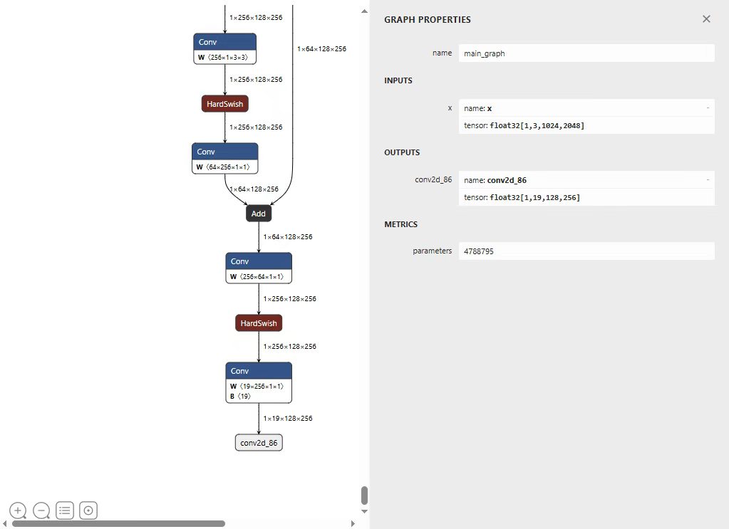
python assets/onnx_export.py --export_path assets/export_models/efficientvit_seg_b1_cityscapes_r1024x2048.onnx --task seg --model efficientvit-seg-b1-cityscapes --resolution 1024 2048 --bs 1使用Netron打开onnx文件,模型输入(1, 3, 1024, 2048) RGB 图,输出:(1, 19, 128, 256) 19 个通道的特征图(logits)
onnx模型测试
导出onnx模型后,加上预处理和后处理操作,对onnx进行推理,不再依赖torch框架(注:在官方模型的训练中,该模型的输入图像是直接resize,没有保持高宽比,此处保持一致)
import cv2
import numpy as np
import onnxruntime as ort

# 配置
IMAGE_PATH = "assets/fig/city.png"
ONNX_PATH = "assets/export_models/efficientvit_seg_b1_cityscapes_r1024x2048.onnx"
OUTPUT_PATH = "output_onnx.png"

INPUT_H = 1024
INPUT_W = 2048
MEAN = np.array([0.485, 0.456, 0.406], dtype=np.float32)
STD = np.array([0.229, 0.224, 0.225], dtype=np.float32)

CITY_COLORS = [
    [128, 64, 128], [244, 35, 232], [70, 70, 70],
    [102, 102, 156], [190, 153, 153], [153, 153, 153],
    [250, 170, 30], [220, 220, 0], [107, 142, 35],
    [152, 251, 152], [70, 130, 180], [220, 20, 60],
    [255, 0, 0], [0, 0, 142], [0, 0, 70],
    [0, 60, 100], [0, 80, 100], [0, 0, 230], [119, 11, 32]
]

def preprocess(image_path):
    img = cv2.imread(image_path)
    img_rgb = cv2.cvtColor(img, cv2.COLOR_BGR2RGB)
    ori_h, ori_w = img_rgb.shape[:2]

    img_rgb = cv2.resize(img_rgb, (INPUT_W, INPUT_H), interpolation=cv2.INTER_AREA)

    img_tensor = img_rgb.astype(np.float32) / 255.0
    img_tensor = (img_tensor - MEAN) / STD
    img_tensor = img_tensor.transpose(2, 0, 1)
    img_tensor = np.expand_dims(img_tensor, axis=0)

    return img_tensor, ori_h, ori_w, img

def postprocess(output_onnx, ori_h, ori_w, ori_img):
    logit = output_onnx[0]
    logit = logit.transpose(1, 2, 0)
    logit = cv2.resize(logit, (INPUT_W, INPUT_H), interpolation=cv2.INTER_LINEAR)
    logit = logit.transpose(2, 0, 1)

    pred_mask = np.argmax(logit, axis=0)
    pred_mask = cv2.resize(pred_mask, (ori_w, ori_h), interpolation=cv2.INTER_NEAREST)

    color_mask = np.zeros((ori_h, ori_w, 3), dtype=np.uint8)
    for idx, c in enumerate(CITY_COLORS):
        color_mask[pred_mask == idx] = c

    color_mask = cv2.cvtColor(color_mask, cv2.COLOR_RGB2BGR)
    final = cv2.addWeighted(ori_img, 0.5, color_mask, 0.5, 0)
    return final, pred_mask

if __name__ == "__main__":
    input_tensor, h, w, ori_img = preprocess(IMAGE_PATH)
    print("输入形状:", input_tensor.shape, " 精度:", input_tensor.dtype)

    session = ort.InferenceSession(ONNX_PATH, providers=["CPUExecutionProvider"])
    output = session.run(None, {session.get_inputs()[0].name: input_tensor})

    # 查看输出
    out = output[0]

    print("输出全局 min = %.6f" % out.min())
    print("输出全局 max = %.6f" % out.max())

    # 打印第一个像素所有通道
    print("第一个像素 (x=0,y=0) 19个通道值:")
    pixel = out[0, :, 0, 0]
    for i, v in enumerate(pixel):
        print(f"类别 {i:2d}: {v:8.3f}")

    print("=" * 60)
    result, pred_mask = postprocess(out, h, w, ori_img)
    print("类别分布:", np.bincount(pred_mask.flatten()))
    cv2.imwrite(OUTPUT_PATH, result)
推理结果出现异常: 
打印onnx推理过程的输出:
输出第一个像素: [nan nan nan nan nan nan nan nan nan nan nan nan nan nan nan nan nan nan nan]
发现onnx输出都是nan,但导出的模型onnx确实是有权重参数,在导出onnx过程打印了如下内容
Obtain model graph for `torch.export.export(..., strict=False)
---->定位问题:PyTorch 2.x 新导出器不兼容 EfficientViT!,有些操作没有正常导出,导致ONNX输出 NAN 。
降级torch版本为2.0.1后,重新导出onnx,推理正常:
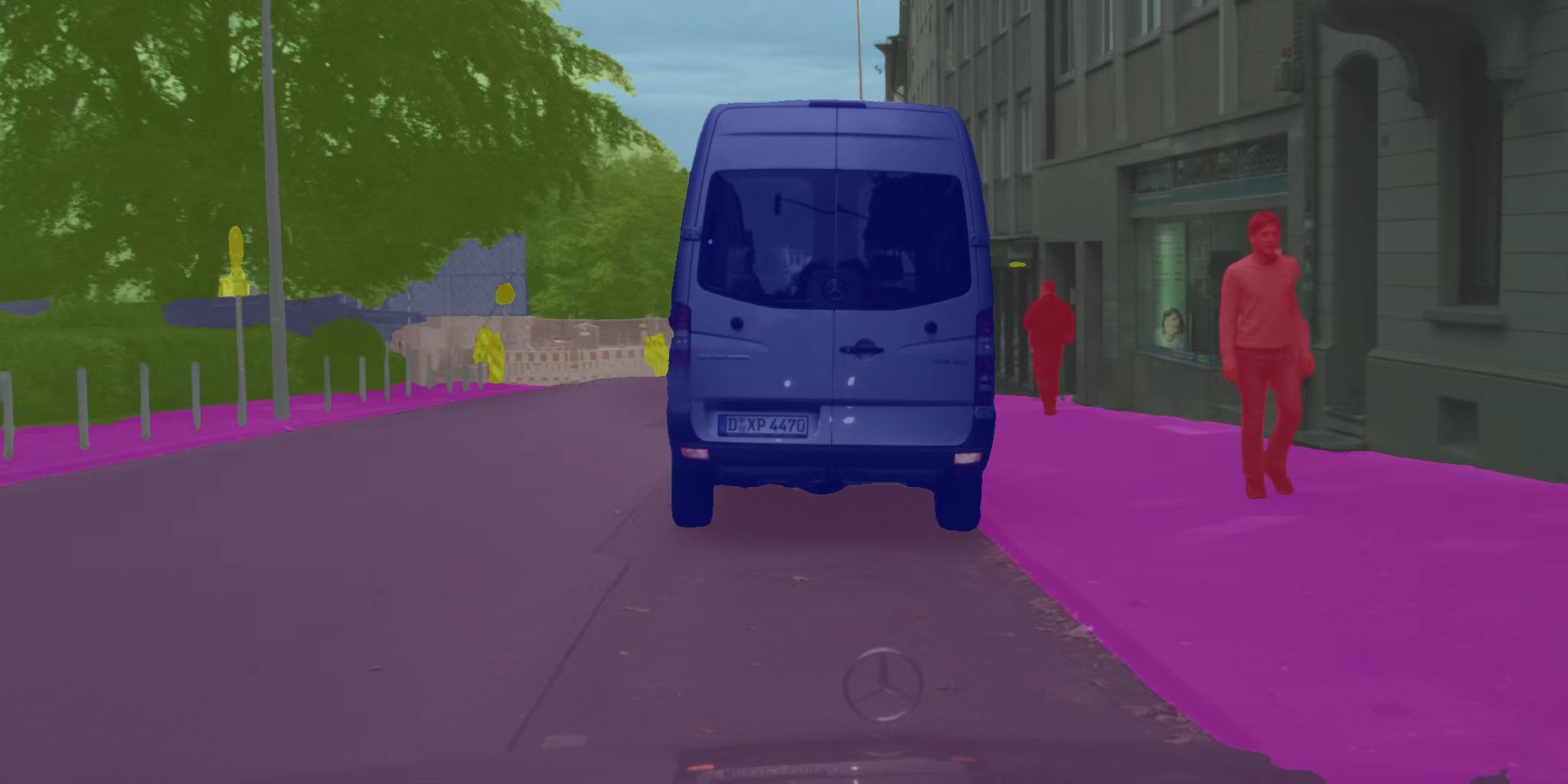
输入形状: (1, 3, 1024, 2048) 精度: float32 输出第一个像素,19个通道值: [-5.024589 -7.6734905 -0.9376892 -5.3960695 -3.7622366 -2.0407202 -1.7906388 -1.7736986 4.07744 -3.7523015 1.0932604 -4.949296 -6.097727 -2.632298 -2.8067648 -5.3893995 -4.2956705 -5.9038606 -6.673056 ] 类别分布:0:625076 1:306627 2:420187 3:24546 4:25459 5:16729 7:5656 8:372128 10:56722 11:35837 13:208185
交叉编译项目构建
基于model_zoo中的examples项目,构建efficientvit_seg,需要修改的内容如下:
cd ./convert_model/修改config_yml.py文件的量化数据集(选取部分cityscapes数据集的训练集),预处理参数。
其中,模型训练的预处理参数为
'mean': [0.485, 0.456, 0.406], 'std': [0.229, 0.224, 0.225]转换后 mean=[0.485, 0.456, 0.406] * 255,scale=1/(std * 255)
# "database"
DATASET = ['../../dataset/cityscapes_10/dataset.txt']
DATASET_TYPE = ["TEXT"]
# mean, scale ##根据模型训练中的图像预处理参数
MEAN = [124, 116, 104]
SCALE = [0.0171, 0.0175, 0.0174]
# reverse_channel: True bgr, False rgb
REVERSE_CHANNEL = False
# add_preproc_node, True or False
ADD_PREPROC_NODE = True
# "preproc_type"
PREPROC_TYPE = ["IMAGE_RGB"]
# add_postproc_node, quant output -> float32 output
ADD_POSTPROC_NODE = True修改model_config.h文件的相关参数配置,定义模型输入尺寸,掩码的色彩
#ifndef _MODEL_CONFIG_H_
#define _MODEL_CONFIG_H_
#include <iostream>
#include <vector>
#include <opencv2/opencv.hpp>

#define Resize_Height	1024
#define Resize_Width	2048

const cv::Vec3b CITY_COLORS[] = {
    {128, 64,128},    // 0
    {244, 35,232},    // 1
    { 70, 70, 70},    // 2
    {102,102,156},    // 3
    {190,153,153},    // 4
    {153,153,153},    // 5
    {250,170, 30},    // 6
    {220,220,  0},    // 7
    {107,142, 35},    // 8
    {152,251,152},    // 9
    { 70,130,180},    // 10
    {220, 20, 60},    // 11
    {255,  0,  0},    // 12
    {  0,  0,142},    // 13
    {  0,  0, 70},    // 14
    {  0, 60,100},    // 15
    {  0, 80,100},    // 16
    {  0,  0,230},    // 17
    {119, 11, 32},    // 18
};
const int NUM_CITY_COLORS = 19;
#endif
模型导入、量化、导出等步骤:(efficientvit_seg_b1_cityscapes_r1024x2048.onnx已重命名为efficientvit_seg.onnx)
# using xxx_env.sh to create softlink
./convert_model_env.sh

# 导入
# pegasus_import.sh <model_name>
./pegasus_import.sh efficientvit_seg

# 量化
# pegasus_quantize.sh <model_name> <quantize_type> <calibration_set_size>
./pegasus_quantize.sh efficientvit_seg int16 10
# 仿真(可选)
# pegasus_inference.sh <model_name> <quantize_type>
./pegasus_inference.sh efficientvit_seg int16

# 导出nb模型
# pegasus_export_ovx_nbg.sh <model_name> <quantize_type> <platform>
./pegasus_export_ovx_nbg.sh efficientvit_seg int16 t736
# 导出的模型文件存放在../model目录
# 例如 ../model/efficientvit_seg_int16_t736.nb
模型输出后处理
模型后处理efficientvit_seg_post.cpp
/*
 * Company:    AW
 * Author:     zhanghuans
 * Date:    2026/5/25
 */
#include <iostream>
#include <vector>
#include <algorithm>
#include <cmath>
#include <cstring>
#include <map>
#include <opencv2/opencv.hpp>
#include <sys/time.h>

#include "model_config.h"

// 处理 NPU 输出 → 生成 pred_mask
static cv::Mat get_pred_mask(const cv::Mat& bgr, float** output)
{
    const int C      = NUM_CITY_COLORS;
    const int H_OUT  = 128;
    const int W_OUT  = 256;
    const int INPUT_H = Resize_Height;
    const int INPUT_W = Resize_Width;

    const float* npu_out = output[0];

    cv::Mat logit_hwc(H_OUT, W_OUT, CV_32FC(C));
    const int HW = H_OUT * W_OUT;
    for (int c = 0; c < C; ++c) {
        float* ptr_channel = logit_hwc.ptr<float>(0) + c;
        for (int i = 0; i < HW; ++i) {
            ptr_channel[i * C] = npu_out[c * HW + i];
        }
    }

    // 上采样)
    cv::Mat resized_logit;
    cv::resize(logit_hwc, resized_logit, cv::Size(INPUT_W, INPUT_H), 0, 0, cv::INTER_LINEAR);

      struct timeval tv1, tv2;
    gettimeofday(&tv1, NULL);

    // argmax
    cv::Mat pred_mask(INPUT_H, INPUT_W, CV_8UC1);
    const float* src = (const float*)resized_logit.data;
    uint8_t* dst = pred_mask.data;

    const int INPUT_HW = INPUT_H * INPUT_W;
    for (int i = 0; i < INPUT_HW; ++i) {
        int max_id = 0;
        float max_score = src[0];

        for (int c = 1; c < C; ++c) {
            if (src[c] > max_score) {
                max_score = src[c];
                max_id = c;
            }
        }

        dst[i] = max_id;
        src += C;
    }

      gettimeofday(&tv2, NULL);
    double total_time_ms = (tv2.tv_sec - tv1.tv_sec) * 1000.0 + (tv2.tv_usec - tv1.tv_usec) / 1000.0;
    fprintf(stderr, "argmax time: %.2f ms\n", total_time_ms);

    return pred_mask;
}


// 处理 pred_mask + 上色、融合、保存
int efficientvit_seg_postprocess(const char *imagepath, float **output)
{
    cv::Mat m = cv::imread(imagepath, 1);
    if (m.empty()) {
        fprintf(stderr, "cv::imread %s failed\n", imagepath);
        return -1;
    }

    struct timeval tv1, tv2;
    gettimeofday(&tv1, NULL);

    // 获取 pred_mask
    cv::Mat pred_mask = get_pred_mask(m, output);

    gettimeofday(&tv2, NULL);
    double total_time_ms = (tv2.tv_sec - tv1.tv_sec) * 1000.0 + (tv2.tv_usec - tv1.tv_usec) / 1000.0;
    fprintf(stderr, "get pred_mask time: %.2f ms\n", total_time_ms);

    /* 调试代码,类别分布
    int cls_count[19] = {0};
    for (int y = 0; y < pred_mask.rows; y++) {
        for (int x = 0; x < pred_mask.cols; x++) {
            int c = pred_mask.at<uint8_t>(y, x);
            if (c >= 0 && c < 19) cls_count[c]++;
        }
    }

    printf("类别分布:");
    for (int i = 0; i < 19; i++) {
        if (cls_count[i] > 0) printf("%d:%d ", i, cls_count[i]);
    }
    printf("\n==================================================\n");
    */

    // 还原原图大小
    cv::Mat final_mask;
    cv::resize(pred_mask, final_mask, m.size(), 0, 0, cv::INTER_NEAREST);

    // 上色
    cv::Mat color_mask(m.size(), CV_8UC3);
    for (int y = 0; y < m.rows; y++) {
        for (int x = 0; x < m.cols; x++) {
            int idx = final_mask.at<uint8_t>(y, x);
            if (idx >= 0 && idx < 19)
                color_mask.at<cv::Vec3b>(y, x) = CITY_COLORS_BGR[idx];
            else
                color_mask.at<cv::Vec3b>(y, x) = {0,0,0};
        }
    }

    // 融合
    cv::addWeighted(m, 0.5, color_mask, 0.5, 0, color_mask);
    cv::imwrite("output_segmentation.png", color_mask);

    fprintf(stderr, "segmentation finished\n");

    return 0;
}
板端demo
含demo编译及运行说明。
解压opencv压缩包
# 进入目录
cd ../../../3rdparty/opencv/
# 解压,选择对应平台
# armhf, eg: V85x, R853
unzip opencv-3.4.16-gnueabihf-linux.zip
# linux aarch64, eg: T527/MR527/MR536/T536/A733/T736
unzip opencv-4.9.0-aarch64-linux-sunxi-glibc.zip
# android aarch64, eg: T527/A733/T736
unzip opencv-4.9.0-android.zip
准备交叉编译工具链
Linux
# 进入目录
cd ../../0-toolchains/
# 解压
# armhf, V85x, R853
unzip arm-openwrt-linux-muslgnueabi.zip
chmod 777 -R ./arm-openwrt-linux-muslgnueabi
# aarch64, MR527, T527, MR536, T536, A733, T736
tar xvf gcc-arm-10.3-2021.07-x86_64-aarch64-none-linux-gnu.tar.xz
# aarch64 for debian11, T527, A733, T736
tar vxf gcc-arm-10.2-2020.11-x86_64-aarch64-none-linux-gnu.tar.xz
build && run
Linux
在Linux系统下测试。编译用法如下:
# 途径一:在centernet目录编译
cd ../examples//efficientvit_seg/
./../build_linux.sh -t <platform> [-s <system>]
# 途径二:在examples目录,再选择centernet目录编译
cd ../examples
./build_linux.sh -t <platform> -p /efficientvit_seg [-s <system>]
以下说明以T736平台为例;
cd ../examples
./build_linux.sh -t t736 -p efficientvit_seg
push 可执行文件、模型文件、输入图片到板端目录;
adb push install/efficientvit_seg_demo_linux_t736 /mnt/UDISK/运行;
adb shell
cd /mnt/UDISK//efficientvit_seg_demo_linux_t736
# 可选
export LD_LIBRARY_PATH=./lib
# 运行可执行文件
# ./centernet_demo_t736 -h 查看执行示例说明
chmod +x ./efficientvit_seg_demo_t736
./efficientvit_seg_demo_t736 -nb model//efficientvit_seg_int16_t736.nb -i model/city.png
exit
adb pull /mnt/UDISK//efficientvit_seg_demo_linux_t736/output_segmentation.png D:/zhanghuans/install/output运行后,打印输出,保存分割结果。
input 0 dim 3 2048 1024 1, data_format=2, quant_format=0, name=input.1_264_out0, none-quant output 0 dim 256 128 19 1, data_format=0, name=uid_1_out_0/out0_0_out0, none-quant nbg name=model//efficientvit_seg_int16_t736.nb, size: 10030512. create network 0: 23366 us. prepare network: 22461 us. buffer ptr: 0xb129300, buffer size: 6291456 feed input cost: 89516 us. network: 0, loop count: 1 run time for this network 0: 566510 us.

免费领 150 小时云算力,进群参与显卡、AI PC 幸运抽奖
更多推荐


 5
5 0
0- 0


 已为社区贡献1条内容

所有评论(0)