1. 数据准备

这里我为大家准备了手写数字图片的数据集MNIST，其中包含了60000个训练样本和10000个测试样本，如下图：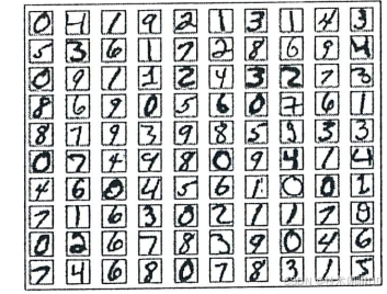

数据集下载链接：https://download.csdn.net/download/wu2374633583/92051855

2. 模型准备和介绍

在此次我们的目的是对图片完成降噪处理，这里我们选的是UNet模型，它的核心任务是学习如何将一张输入图像（如手写数字）转换成一张有特定含义的输出图像。
后续我会深入讲模型的选型问题。

2.1 模型下载

链接：https://download.csdn.net/download/wu2374633583/92051862

2.2 模型定义代码

unet.py类

import numpy as np
import torch

# x_train = np.load('./mnist/x_train.npy')
# y_train = np.load('./mnist/y_train_label.npy')
# print(x_train.shape)

class Unet(torch.nn.Module):
    def __init__(self):
        super(Unet, self).__init__()
        # 模块化结构，这也是后面常用到的模型结构
        self.first_block_down = torch.nn.Sequential(
            torch.nn.Conv2d(in_channels=1, out_channels=32, kernel_size=3, padding=1), torch.nn.GELU(),
            torch.nn.MaxPool2d(kernel_size=2, stride=2)
        )

        self.second_block_down = torch.nn.Sequential(
            torch.nn.Conv2d(in_channels=32, out_channels=64, kernel_size=3, padding=1), torch.nn.GELU(),
            torch.nn.MaxPool2d(kernel_size=2, stride=2)
        )

        self.latent_space_block = torch.nn.Sequential(
            torch.nn.Conv2d(in_channels=64, out_channels=128, kernel_size=3, padding=1), torch.nn.GELU(),
        )

        self.second_block_up = torch.nn.Sequential(
            torch.nn.Upsample(scale_factor=2),
            torch.nn.Conv2d(in_channels=128, out_channels=64, kernel_size=3, padding=1), torch.nn.GELU(),
        )

        self.first_block_up = torch.nn.Sequential(
            torch.nn.Upsample(scale_factor=2),
            torch.nn.Conv2d(in_channels=64, out_channels=32, kernel_size=3, padding=1), torch.nn.GELU(),
        )

        self.convUP_end = torch.nn.Sequential(
            torch.nn.Conv2d(in_channels=32, out_channels=1, kernel_size=3, padding=1),
            torch.nn.Tanh()
        )

    def forward(self,img_tensor):
        image = img_tensor

        image = self.first_block_down(image)#;print(image.shape)     # torch.Size([5, 32, 14, 14])
        image = self.second_block_down(image)#;print(image.shape)    # torch.Size([5, 16, 7, 7])
        image = self.latent_space_block(image)#;print(image.shape)   # torch.Size([5, 8, 7, 7])

        image = self.second_block_up(image)#;print(image.shape)      # torch.Size([5, 16, 14, 14])
        image = self.first_block_up(image)#;print(image.shape)       # torch.Size([5, 32, 28, 28])
        image = self.convUP_end(image)#;print(image.shape)           # torch.Size([5, 32, 28, 28])
        return image


if __name__ == '__main__':
    image = torch.randn(size=(5,1,28,28))
    unet_model = Unet()
    torch.save(unet_model, './unet_model.pth')

2.3 模型架构解读

U-Net模型的核心是一个编码器-解码器结构，形状像字母“U”。

• 编码器（下采样路径）​​：first_block_down和second_block_down模块负责此项工作。它们通过卷积层提取图像特征，再通过池化层压缩图像尺寸。这个过程可以理解为不断“抓住”图像中最重要的信息（比如物体的轮廓、纹理），但会忽略一些细节。

• 瓶颈层​：latent_space_block是连接编码器和解码器的关键部分。它处理的是被高度压缩后的信息，这些信息包含了图像最核心、最抽象的语义特征。

• 解码器（上采样路径）​​：second_block_up和first_block_up模块负责此项工作。它们通过上采样操作将特征图的尺寸逐步放大，恢复细节，最终目标是还原到输入图像的尺寸。

2.4 关键组件与数据流

在 forward函数中，你可以清晰地看到一张图像是如何流经这个模型的：

def forward(self, img_tensor):
    image = img_tensor  # 输入图像，尺寸为 [批次大小, 通道数, 高, 宽]，例如 [5, 1, 28, 28]
    image = self.first_block_down(image)   # 下采样 -> [5, 32, 14, 14]
    image = self.second_block_down(image)  # 下采样 -> [5, 64, 7, 7]
    image = self.latent_space_block(image)  # 特征提取 -> [5, 128, 7, 7]
    image = self.second_block_up(image)    # 上采样 -> [5, 64, 14, 14]
    image = self.first_block_up(image)     # 上采样 -> [5, 32, 28, 28]
    image = self.convUP_end(image)         # 输出层 -> [5, 1, 28, 28]
    return image

输出层使用的 Tanh()激活函数会将每个像素的值压缩到 ​​-1 到 1​ 的范围内。这表明该模型可能用于图像生成或去噪等任务，需要输出像素值范围较广的图像，而不是像分割任务那样输出概率。

2.5 典型应用场景

基于其结构，这个模型可能用于以下任务：​

• 图像分割​：尤其是医学影像（细胞、器官）、卫星图像分析或道路裂纹检测。

• 图像生成与重建​：由于输出使用了 Tanh，也可能用于简单的图像生成或去噪任务。

3. 对目标的逼近-模型的损失函数和优化函数

要完成一个深度学习项目，一个非常重要的内容就是设定模型的损失函数和优化函数。这里我们采用的是均方损失函数MSELoss。它的作用就是计算预测值和真实值之间的欧氏距离，二者越接近，均方差就越小。

4. 基于深度学习模型训练

4.1 完整代码

import os

os.environ['CUDA_VISIBLE_DEVICES'] = '0'
import torch
import numpy as np
import unet
import matplotlib.pyplot as plt
from tqdm import tqdm

# 创建保存图像的目录
img_dir = "./img"
if not os.path.exists(img_dir):
    os.makedirs(img_dir)
    print(f"创建目录: {img_dir}")

batch_size = 320                        #设定每次训练的批次数
epochs = 1024                           #设定训练次数

#device = "cpu"                         #Pytorch的特性，需要指定计算的硬件，如果没有GPU的存在，就使用CPU进行计算
device = "cuda"                         #在这里读者默认使用GPU，如果读者出现运行问题可以将其改成cpu模式

model = unet.Unet()                     #导入Unet模型
model = model.to(device)                #将计算模型传入GPU硬件等待计算
#model = torch.compile(model)            #Pytorch2.0的特性，加速计算速度 选择使用内容
optimizer = torch.optim.Adam(model.parameters(), lr=2e-5)   #设定优化函数

#载入数据
x_train = np.load("./mnist/x_train.npy")
y_train_label = np.load("./mnist/y_train_label.npy")

x_train_batch = []
for i in range(len(y_train_label)):
    if y_train_label[i] <= 10:                    #为了加速演示作者只对数据集中的小于2的数字，也就是0和1进行运行，读者可以自行增加训练个数
        x_train_batch.append(x_train[i])

x_train = np.reshape(x_train_batch, [-1, 1, 28, 28])  #修正数据输入维度：([30596, 28, 28])
x_train /= 512.
train_length = len(x_train) * 20                       #增加数据的单词循环次数

#state_dict = torch.load("./saver/unet.pth")
#model.load_state_dict(state_dict)
for epoch in range(30):
    train_num = train_length // batch_size             #计算有多少批次数

    train_loss = 0                                     #用于损失函数的统计
    for i in tqdm(range(train_num)):                    #开始循环训练
        x_imgs_batch = []                               #创建数据的临时存储位置
        x_step_batch = []
        y_batch = []
        # 对每个批次内的数据进行处理
        for b in range(batch_size):
            img = x_train[np.random.randint(x_train.shape[0])]  #提取单个图片内容
            x = img
            y = img

            x_imgs_batch.append(x)
            y_batch.append(y)

        #将批次数据转化为Pytorch对应的tensor格式并将其传入GPU中
        x_imgs_batch = torch.tensor(x_imgs_batch).float().to(device)
        y_batch = torch.tensor(y_batch).float().to(device)


        pred = model(x_imgs_batch)                      #对模型进行正向计算
        loss = torch.nn.MSELoss(reduction="sum")(pred, y_batch)*100.   #使用损失函数进行计算

        #这里读者记住下面就是固定格式，一般而言这样使用即可
        optimizer.zero_grad()                                               #对结果进行优化计算
        loss.backward()                                                     #损失值的反向传播
        optimizer.step()                                                    #对参数进行更新

        train_loss += loss.item()                                           #记录每个批次的损失值
    #计算并打印损失值
    train_loss /= train_num
    print("train_loss:", train_loss)
    if epoch%6 == 0:
        torch.save(model.state_dict(),"./unet_model.pth")

    # 下面是对数据进行打印
    image = x_train[np.random.randint(x_train.shape[0])]
    image = np.reshape(image, [1, 1, 28, 28])

    image = torch.tensor(image).float().to(device)
    image = model(image)

    image = torch.reshape(image, shape=[28, 28])
    image = image.detach().cpu().numpy()

    # 保存图像 - 现在目录已经存在
    plt.imshow(image)
    plt.savefig(f"./img/img_{epoch}.jpg")

4.2 代码解读

1、环境设置与导入模块

import os
os.environ['CUDA_VISIBLE_DEVICES'] = '0'  # 设置使用哪个GPU
import torch
import numpy as np
import unet  # 自定义的U-Net模型
import matplotlib.pyplot as plt
from tqdm import tqdm  # 进度条工具

• 配置计算环境，优先使用GPU（CUDA）加速训练
• 导入必要的深度学习库：PyTorch用于张量计算，NumPy用于数值处理，matplotlib用于可视化

2、创建输出目录

img_dir = "./img"
if not os.path.exists(img_dir):
    os.makedirs(img_dir)
    print(f"创建目录: {img_dir}")

• os.path.exists()和 os.makedirs()是文件系统操作，类似Java的File.exists()和File.mkdirs()

• f"字符串{变量}"是f-string格式，Python 3.6+的特性。

3、超参数设置与设备选择

batch_size = 320    # 每次训练输入的样本数
epochs = 1024       # 训练轮数
device = "cuda"     # 使用GPU加速

• Batch Size: 一次迭代中处理的样本数量，影响训练速度和内存使用。
• Epoch: 整个训练数据集被完整遍历一次的计数。
• GPU加速: 使用CUDA可以大幅提升矩阵运算速度，这对深度学习至关重要。

4、模型初始化

model = unet.Unet()                    # 实例化U-Net模型
model = model.to(device)               # 将模型移至GPU
optimizer = torch.optim.Adam(model.parameters(), lr=2e-5)  # 优化器

• Adam优化器自适应调整学习率，比传统梯度下降更高效。学习率lr=2e-5控制参数更新步长。

5、数据加载与预处理

x_train = np.load("./mnist/x_train.npy")  # 加载训练数据
y_train_label = np.load("./mnist/y_train_label.npy")  # 加载标签

# 过滤数据，只使用标签<=10的样本
x_train_batch = []
for i in range(len(y_train_label)):
    if y_train_label[i] <= 10:
        x_train_batch.append(x_train[i])

# 数据重塑和归一化
x_train = np.reshape(x_train_batch, [-1, 1, 28, 28])  # 调整维度
x_train /= 512.  # 像素值归一化到[0,1]范围
train_length = len(x_train) * 20  # 增加数据循环次数

• 维度调整: reshape([-1, 1, 28, 28])将数据变为(batch_size, 通道数, 高度,宽度)格式，PyTorch需要此格式。
• 数据归一化: 将像素值从0-255缩放到0-1之间，提高训练稳定性和收敛速度。
• ​数据过滤: 只使用部分类别（0-10）加速演示训练过程。

6、训练循环核心逻辑

for epoch in range(30):  # 外层训练循环
    train_num = train_length // batch_size  # 计算批次数
    
    train_loss = 0
    for i in tqdm(range(train_num)):  # 进度条显示
        # 准备批次数据
        x_imgs_batch = []
        y_batch = []
        for b in range(batch_size):
            img = x_train[np.random.randint(x_train.shape[0])]  # 随机采样
            x_imgs_batch.append(img)
            y_batch.append(img)  # 本例中输入和目标相同（自编码器任务）
        
        # 转换为PyTorch张量并移至GPU
        x_imgs_batch = torch.tensor(x_imgs_batch).float().to(device)
        y_batch = torch.tensor(y_batch).float().to(device)
        
        # 前向传播
        pred = model(x_imgs_batch)
        loss = torch.nn.MSELoss(reduction="sum")(pred, y_batch) * 100.
        
        # 反向传播与优化
        optimizer.zero_grad()  # 清零梯度
        loss.backward()        # 计算梯度
        optimizer.step()       # 更新参数
        
        train_loss += loss.item()  # 累积损失

训练过程详解​：

• 前向传播​：输入数据通过模型计算预测输出 ​损失计算​：使用均方误差（MSE）
• 衡量预测与真实值的差异
• 反向传播​：自动计算损失函数对模型参数的梯度 ​
• 参数更新​：优化器根据梯度更新模型权重

7、 模型保存与结果可视化

# 定期保存模型
if epoch % 6 == 0:
    torch.save(model.state_dict(), "./unet_model.pth")

# 生成示例图像
image = x_train[np.random.randint(x_train.shape[0])]
image = np.reshape(image, [1, 1, 28, 28])
image = torch.tensor(image).float().to(device)
image = model(image)  # 模型推理

# 结果可视化
image = torch.reshape(image, shape=[28, 28])
image = image.detach().cpu().numpy()  # 移回CPU并转NumPy
plt.imshow(image)
plt.savefig(f"./img/img_{epoch}.jpg")

模型保存机制​：

• model.state_dict()保存模型参数而非整个模型，便于跨平台部署
• PyTorch的.pth文件包含张量字典，类似Java的序列化对象

可视化重要性​：

• 深度学习训练中，可视化帮助监控模型表现，检测训练问题。这里每6个epoch保存一次生成图像。

4.3 最后训练效果展示

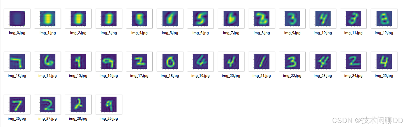
从图中我们可以看到，随着模型的训练，它逐渐学会了对输入数据进行整形和输出。