
MPC模型预测控制
这篇主要讲一下模型预测控制,如果对PID控制了解的同学,那效果更好。如果不了解PID控制,还是熟悉下比较好。模型预测控制,顾名思义,基于模型,预测未来,进行控制。这个控制是基于模型的,也就是model-based。有人会问,我这个系统的模型怎么来呢?我想到两点解决方法:1. 文献上去找别人已经建好的,公认的模型;2. 首先进行系统辨识,再进行建模。(难度太大,不建议)下面给上经...
这篇主要讲一下模型预测控制,如果对PID控制了解的同学,那效果更好。如果不了解PID控制,还是熟悉下比较好。
模型预测控制,顾名思义,基于模型,预测未来,进行控制。这个控制是基于模型的,也就是model-based。
有人会问,我这个系统的模型怎么来呢?我想到两点解决方法:
1. 文献上去找别人已经建好的,公认的模型;
2. 首先进行系统辨识,再进行建模。(难度太大,不建议)
下面给上经典的MPC控制流程图:
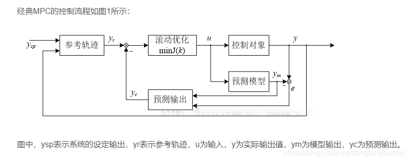
模型预测控制是一种基于模型的闭环优化控制策略。
预测控制算法的三要素:内部(预测)模型、参考轨迹、控制算法。现在一般则更清楚地表述为内部(预测)模型、滚动优化、反馈控制。
大量的预测控制权威性文献都无一例外地指出, 预测控制最大的吸引力在于它具有显式处理约束的能力, 这种能力来自其基于模型对系统未来动态行为的预测, 通过把约束加到未来的输入、输出或状态变量上, 可以把约束显式表示在一个在线求解的二次规划或非线性规划问题中.
模型预测控制具有控制效果好、鲁棒性强等优点,可有效地克服过程的不确定性、非线性和并联性,并能方便的处理过程被控变量和操纵变量中的各种约束。[1]
在线性模型预测控制(Linear Model Predictive Control, LMPC)的基础上,发展了非线性模型预测控制(Non-linear Model Predictive Control, NMPC),显示模型预测控制(Explicit Model Predictive Control, EMPC)和 鲁棒模型预测控制(Robust Model Predictive Control)
首先,我们定义一个模型来描述我们的车辆。[2]
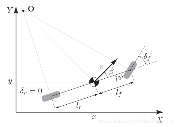
这是自行车模型,运动学上面经常使用。
(x, y)是车辆的质心,ψ是当前车身的角度,v是当前车辆的速度,lf是当前车辆质心到原点的距离, β是速度和车身的角度。在我们的例子中,我们假设β为零,也就是没有侧滑。
在我们的模型中,我们可以通过控制前轮的转角δf 以及车辆的加速度a来控制车辆轨迹。简单起见,我们只考虑前轮驱动的车辆,并且将δf记作δ。
模型预测控制的细节
每个控制周期,我们都从传感器读取数据并得到车辆状态量:
-
车辆的位置(x,y)
-
速度v
-
车身角度 ψ
-
转向角(舵角) δ
-
加速度a
轨迹模型:
我们的道路检测系统应该能够为我们规划好路线,比如,以接下来6个航点的坐标的形式。在我们的例子中,我们使用6个航点去逼近一个3阶多项式函数。我们用这个模型去计算y坐标和相对于x轴的车身角度ψ。

轨迹模型一般有规划模块给出,在这里就不做深入的研究。
动态模型:
接下来,我们要创建动态模型利用t时刻的状态去预测在t+1拍时刻的车辆状态。利用动力学模型,我们可以轻易地从最新时刻地采样推导出下一时刻的位置,车身角度和速度。

我们可以在添加另外2个状态去衡量轨迹跟踪误差和车身角度误差ψ:

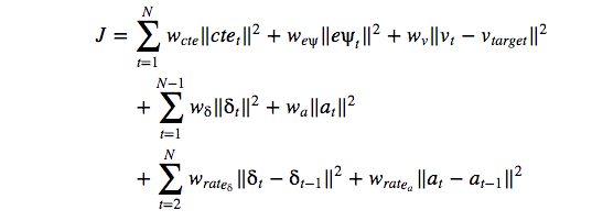
损失函数:
在模型预测控制中,我们需要定义损失函数来优化路径。如果模型不能保持目标速度,那么我们就要惩罚模型。如果可能的话,我们并不想要突然的加减速或者突然的转向。但是既然这些实际上是不可避免的,我们可以尽可能地抑制加减速和转向地变化率。这减轻了晕车同时更加省油(也省人民币)。模型的损失函数应当包含
-
跟踪误差
-
转向误差
-
速度损失函数项(尽量保持在100英里每小时)
-
转向损失函数项(尽量避免转向)
-
加速度损失函数项(尽量保持0加速度)
-
转向变化率(越小越好)
-
加速度变化率(越小越好)
因为这些目标也许会相互冲突,我们需要给这些损失项定义权重以体现优先级。损失函数如下:
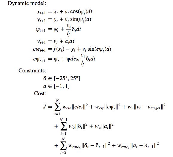
总而言之:
我们需要用模型预测控制来寻找最优路径,那么就需要动力学模型来预测下一拍的状态,以下是动力学模型和系统约束:
这是下面GitHub链接里,别人给的权重。
    const int cte_cost_weight = 2000;
    const int epsi_cost_weight = 2000;
    const int v_cost_weight = 1;
    const int delta_cost_weight = 10;
    const int a_cost_weight = 10;
    const int delta_change_cost_weight = 100;
    const int a_change_cost_weight = 10;
优化模型预测控制
我们通过解决一个约束条件下优化损失函数的问题来解决了控制问题。这些约束条件包括油门和转向的控制。
-
从道路中检测下6个航点,并且计算3次插值的来建立行驶轨迹
-
从传感器读取当前速度v, 方向ψ, 转向角 δ 以及加速度 a
-
使用传感器读取的数据和动力学模型计算出第一个车辆状态
-
根据1秒内的车辆状态响应优化控制动作,控制的周期为100ms,所以1s内有10个周期
-
模型预测控制的两个变量(也是控制量):加速度(油门对应正加速度,刹车对应负加速度)和转向角
-
给出加速度和转向角的约束范围
-
我们将动态模型计算9次,得到未来9个时间拍的系统状态
-
给出每个采样计算周期的损失函数
-
用1个优化器解算出在约束定义下周期1到周期9的最小总损失(注意,在我们的定义中,时间周期并不从0开始,而是从1开始到10)
-
我们仅仅选择周期1给出的控制量
-
但是,我们延时100ms后再将控制量给模拟器。这样能够模拟现实世界,毕竟处理计算(读取传感器)和执行都需要时间。
-
从步骤1开始重复,寻找下一个最优控制量。
可调性:
在我们的例子中,我们计算了1秒中内的最优解,这个参数是可以调节的。长时间窗口的优化会给控制器的动作漂亮的曲线,但是也会积累过多的误差。实际上,如果这个优化时间窗口太大,汽车反而会脱离期望轨迹。
上面的文章内容都来自于链接[2]中,但是很多人对MPC还是有点不明白。模型也建立好了,约束我也会给,那怎么求解呢?求的解怎么利用呢?
现在我们看第一个问题:
1. 如何求解
上面的文章其实来自于Udacity的自动驾驶的一个课程。
大家可以去GitHub上下载下来,自己跑一下上面的代码。链接是这个https://github.com/mvirgo/MPC-Project,里面是一位博主写好的代码。大家配置好环境后可以直接跑起来的,然后有个可视化软件,可以看到3D引擎看到动画。
比如像这样的:https://github.com/mvirgo/MPC-Project/blob/master/MPC_vid.mov。
这个代码尽量在Ubuntu上去跑,因为装的东西比较多,给的教程关于LInux的。教程还是看Udacity给的模板比较好,但是代码不要下这个网址的,当时我环境配置好了之后还是有报错,我还以为是我环境配置的有问题。https://github.com/udacity/CarND-MPC-Project
这个代码是C++写的。
主函数中的调用
 /*
          * Calculate steering angle and throttle using MPC.
          * Both are in between [-1, 1].
          * Simulator has 100ms latency, so will predict state at that point in time.
          * This will help the car react to where it is actually at by the point of actuation.
          */

          // Fits a 3rd-order polynomial to the above x and y coordinates
          auto coeffs = polyfit(ptsx_car, ptsy_car, 3);

          // Calculates the cross track error
          // Because points were transformed to vehicle coordinates, x & y equal 0 below.
          // 'y' would otherwise be subtracted from the polyeval value
          double cte = polyeval(coeffs, 0);

          // Calculate the orientation error
          // Derivative of the polyfit goes in atan() below
          // Because x = 0 in the vehicle coordinates, the higher orders are zero
          // Leaves only coeffs[1]
          double epsi = -atan(coeffs[1]);

          // Center of gravity needed related to psi and epsi
          const double Lf = 2.67;

          // Latency for predicting time at actuation
          const double dt = 0.1;

          // Predict state after latency
          // x, y and psi are all zero after transformation above
          double pred_px = 0.0 + v * dt; // Since psi is zero, cos(0) = 1, can leave out
          const double pred_py = 0.0; // Since sin(0) = 0, y stays as 0 (y + v * 0 * dt)
          double pred_psi = 0.0 + v * -delta / Lf * dt;
          double pred_v = v + a * dt;
          double pred_cte = cte + v * sin(epsi) * dt;
          double pred_epsi = epsi + v * -delta / Lf * dt;

          // Feed in the predicted state values
          Eigen::VectorXd state(6);
          state << pred_px, pred_py, pred_psi, pred_v, pred_cte, pred_epsi;

          // Solve for new actuations (and to show predicted x and y in the future)
          auto vars = mpc.Solve(state, coeffs);

          // Calculate steering and throttle
          // Steering must be divided by deg2rad(25) to normalize within [-1, 1].
          // Multiplying by Lf takes into account vehicle's turning ability
          double steer_value = vars[0] / (deg2rad(25) * Lf);
          double throttle_value = vars[1];
MPC函数的实现
// MPC class definition implementation.
//
MPC::MPC() {}
MPC::~MPC() {}

vector<double> MPC::Solve(Eigen::VectorXd state, Eigen::VectorXd coeffs) {
  bool ok = true;
  typedef CPPAD_TESTVECTOR(double) Dvector;

  // State vector holds all current values neede for vars below
  double x = state[0];
  double y = state[1];
  double psi = state[2];
  double v = state[3];
  double cte = state[4];
  double epsi = state[5];

  // Setting the number of model variables (includes both states and inputs).
  // N * state vector size + (N - 1) * 2 actuators (For steering & acceleration)
  size_t n_vars = N * 6 + (N - 1) * 2;
  // Setting the number of constraints
  size_t n_constraints = N * 6;

  // Initial value of the independent variables.
  // SHOULD BE 0 besides initial state.
  Dvector vars(n_vars);
  for (int i = 0; i < n_vars; i++) {
    vars[i] = 0.0;
  }

  Dvector vars_lowerbound(n_vars);
  Dvector vars_upperbound(n_vars);
  // Sets lower and upper limits for variables.
  // Set all non-actuators upper and lowerlimits
  // to the max negative and positive values.
  for (int i = 0; i < delta_start; i++) {
    vars_lowerbound[i] = -1.0e19;
    vars_upperbound[i] = 1.0e19;
  }

  // The upper and lower limits of delta are set to -25 and 25
  // degrees (values in radians).
  for (int i = delta_start; i < a_start; i++) {
    vars_lowerbound[i] = -0.436332;
    vars_upperbound[i] = 0.436332;
  }

  // Acceleration/decceleration upper and lower limits.
  for (int i = a_start; i < n_vars; i++) {
    vars_lowerbound[i] = -1.0;
    vars_upperbound[i] = 1.0;
  }

  // Lower and upper limits for the constraints
  // Should be 0 besides initial state.
  Dvector constraints_lowerbound(n_constraints);
  Dvector constraints_upperbound(n_constraints);
  for (int i = 0; i < n_constraints; i++) {
    constraints_lowerbound[i] = 0;
    constraints_upperbound[i] = 0;
  }

  // Start lower and upper limits at current values
  constraints_lowerbound[x_start] = x;
  constraints_lowerbound[y_start] = y;
  constraints_lowerbound[psi_start] = psi;
  constraints_lowerbound[v_start] = v;
  constraints_lowerbound[cte_start] = cte;
  constraints_lowerbound[epsi_start] = epsi;

  constraints_upperbound[x_start] = x;
  constraints_upperbound[y_start] = y;
  constraints_upperbound[psi_start] = psi;
  constraints_upperbound[v_start] = v;
  constraints_upperbound[cte_start] = cte;
  constraints_upperbound[epsi_start] = epsi;

  // object that computes objective and constraints
  FG_eval fg_eval(coeffs);

  //
  // NOTE: You don't have to worry about these options
  //
  // options for IPOPT solver
  std::string options;
  // Uncomment this if you'd like more print information
  options += "Integer print_level  0\n";
  // NOTE: Setting sparse to true allows the solver to take advantage
  // of sparse routines, this makes the computation MUCH FASTER. If you
  // can uncomment 1 of these and see if it makes a difference or not but
  // if you uncomment both the computation time should go up in orders of
  // magnitude.
  options += "Sparse  true        forward\n";
  options += "Sparse  true        reverse\n";
  // NOTE: Currently the solver has a maximum time limit of 0.5 seconds.
  // Change this as you see fit.
  options += "Numeric max_cpu_time          0.5\n";

  // place to return solution
  CppAD::ipopt::solve_result<Dvector> solution;

  // solve the problem
  CppAD::ipopt::solve<Dvector, FG_eval>(
      options, vars, vars_lowerbound, vars_upperbound, constraints_lowerbound,
      constraints_upperbound, fg_eval, solution);

  // Check some of the solution values
  ok &= solution.status == CppAD::ipopt::solve_result<Dvector>::success;

  // Cost
  auto cost = solution.obj_value;
  std::cout << "Cost " << cost << std::endl;

  // Return the first actuator values, along with predicted x and y values to plot in the simulator.
  vector<double> solved;
  solved.push_back(solution.x[delta_start]);
  solved.push_back(solution.x[a_start]);
  for (int i = 0; i < N; ++i) {
    solved.push_back(solution.x[x_start + i]);
    solved.push_back(solution.x[y_start + i]);
  }

  return solved;

}
具体源码大家还是去直接下载代码看看看。跑下看看效果。然后可以改下预测步长N和采样周期t。这里给的N=10,t=0.1s。
大家有什么问题,我们可以一起交流下,相互促进,共同进步。我C++一般,是硬伤,Linux也是用了没多久,就为了跑这个工程。
如何求解的问题已经解决。
2. 如何利用
如何利用比求解简单多了啊,看代码:
// Send values to the simulator
          json msgJson;
          msgJson["steering_angle"] = steer_value;
          msgJson["throttle"] = throttle_value;

          // Display the MPC predicted trajectory
          vector<double> mpc_x_vals = {state[0]};
          vector<double> mpc_y_vals = {state[1]};

          // add (x,y) points to list here, points are in reference to the vehicle's coordinate system
          // the points in the simulator are connected by a Green line

          for (int i = 2; i < vars.size(); i+=2) {
            mpc_x_vals.push_back(vars[i]);
            mpc_y_vals.push_back(vars[i+1]);
          }

          msgJson["mpc_x"] = mpc_x_vals;
          msgJson["mpc_y"] = mpc_y_vals;

          // Display the waypoints/reference line
          vector<double> next_x_vals;
          vector<double> next_y_vals;

          // add (x,y) points to list here, points are in reference to the vehicle's coordinate system
          // the points in the simulator are connected by a Yellow line
          double poly_inc = 2.5;
          int num_points = 25;

          for (int i = 1; i < num_points; i++) {
            next_x_vals.push_back(poly_inc * i);
            next_y_vals.push_back(polyeval(coeffs, poly_inc * i));
          }

          msgJson["next_x"] = next_x_vals;
          msgJson["next_y"] = next_y_vals;

          auto msg = "42[\"steer\"," + msgJson.dump() + "]";
          std::cout << msg << std::endl;
          // Latency
          // The purpose is to mimic real driving conditions where
          // the car doesn't actuate the commands instantly.
          this_thread::sleep_for(chrono::milliseconds(100));
          ws.send(msg.data(), msg.length(), uWS::OpCode::TEXT);
        }
      } else {
        // Manual driving
        std::string msg = "42[\"manual\",{}]";
        ws.send(msg.data(), msg.length(), uWS::OpCode::TEXT);
      }
主要看前两句,就是把计算好的发送到模拟器,实际的话应该是发信号给方向盘和脚踏板。还有预测的轨迹点也输出到模拟器。
现在大家再看看链接[2]中的这段话,是不是有点感觉:
自动驾驶的3大核心科技是定位(在哪里),感知(周围是啥)以及控制(咋开车呢)。通过车道检测,我们可以对车的行进路线进行路径规划。本篇文章主要通过一个自行车的动力学模型讨论车辆的加速、刹车和转向的模型预测控制。目的不仅在于尽可能地控制车辆轨迹,同时也还要尽可能使速度平滑以避免晕车和频繁的刹车。
模型预测控制主要在约束条件下使损失函数最小。例如,我们想要以100ms的周期调整转向和速度,在转向角度不能超过25°的约束下,最小化以规划的路径和实际路径之间的误差。我们通过传感器获取车辆的状态,比如速度,而我们的动作基于传感器读数以一个短的周期执行(例如1s)。例如,我们顺时针转向20°,然后每100ms周期减小1°。加入这些动作可以1秒钟之后的损失函数最小,我们将会采用第一个动作:顺时针转动20°,但是却并不执行后续的动作,而是在100ms后,重复优化过程。100ms后,有了新的读数,我们就重新计算下一个最优动作。模型预测控制通过预测接下来一段较长时间(1s)的损失函数,来计算选择出下一个较短周期(100ms)的最优动作。相比于短视的贪心算法,模型预测控制具有鲁棒性,因此能够控制得更好。
给出一张图,大家可能看的更明白了。

这是维基百科上的图[3]。
这一篇就到这里吧,写的也不够深入,下一篇我会讲MATLAB中的实现。感谢下以下三个链接的作者。
[1] https://www.cnblogs.com/kui-sd具体u/p/9026796.html
[2] https://www.leiphone.com/news/201812/3iia3PiNHnHiUFMb.html(中文翻译)
[3] https://zh.wikipedia.org/wiki/%E6%A8%A1%E5%9E%8B%E9%A0%90%E6%B8%AC%E6%8E%A7%E5%88%B6

旨在为数千万中国开发者提供一个无缝且高效的云端环境,以支持学习、使用和贡献开源项目。
更多推荐


 161
161 0
0- 0


 已为社区贡献3条内容

所有评论(0)