【机器学习】NMF(非负矩阵分解)
写在篇前 本篇文章主要介绍NMF算法原理以及使用sklearn中的封装方法实现该算法,最重要的是理解要NMF矩阵分解的实际意义,将其运用到自己的数据分析中!理论概述 NMF(Non-negative matrix factorization),即对于任意给定的一个非负矩阵V,其能够寻找到一个非负矩阵W和一个非负矩阵H,满足条件V=W*H,从而将一个非负的矩阵分解为左右两个非负矩阵的乘积。...
写在篇前
本篇文章主要介绍NMF算法原理以及使用sklearn中的封装方法实现该算法,最重要的是理解要NMF矩阵分解的实际意义,将其运用到自己的数据分析中!
理论概述
NMF(Non-negative matrix factorization),即对于任意给定的一个非负矩阵V,其能够寻找到一个非负矩阵W和一个非负矩阵H,满足条件V=W*H,从而将一个非负的矩阵分解为左右两个非负矩阵的乘积。**其中,V矩阵中每一列代表一个观测(observation),每一行代表一个特征(feature);W矩阵称为基矩阵,H矩阵称为系数矩阵或权重矩阵。这时用系数矩阵H代替原始矩阵,就可以实现对原始矩阵进行降维,得到数据特征的降维矩阵,从而减少存储空间。**过程如下图所示:

nmf更详尽的原理可以参考Non-negative matrix factorization - Wikipedia,这里我主要列出我很关注的损失函数(lossFunction or objective function):
-
squared frobenius norm
a r g    m i n ⎵ W , H 1 2 ∣ ∣ A − W H ∣ ∣ F r o 2 + α ρ ∣ ∣ W ∣ ∣ 1 + α ρ ∣ ∣ H ∣ ∣ 1 + α ( 1 − ρ ) 2 ∣ ∣ W ∣ ∣ F r o 2 + α ( 1 − ρ ) 2 ∣ ∣ H ∣ ∣ F r o 2 \underbrace{arg\;min}_{W,H}\frac{1}{2}||A-WH||_{Fro}^2 +\alpha\rho|| W||_1+\alpha\rho|| H||_1+\frac{\alpha(1-\rho)}{2}|| W||_{Fro}^2 + \frac{\alpha(1-\rho)}{2}|| H||_{Fro}^2 W,H argmin21∣∣A−WH∣∣Fro2+αρ∣∣W∣∣1+αρ∣∣H∣∣1+2α(1−ρ)∣∣W∣∣Fro2+2α(1−ρ)∣∣H∣∣Fro2
其中:
1 2 ∣ ∣ A − W H ∣ ∣ F r o 2 = 1 2 ∑ i , j ( A i j − W H i j ) 2 \frac{1}{2} ||A - WH||_{\mathrm{Fro}}^2 = \frac{1}{2} \sum_{i,j} (A_{ij} - {WH}_{ij})^2 21∣∣A−WH∣∣Fro2=21i,j∑(Aij−WHij)2
α \alpha α为L1&L2正则化参数,而\rho为L1正则化占总正则化项的比例。||*||_1为L1范数。 -
Kullback-Leibler (KL)
d K L ( X , Y ) = ∑ i , j ( X i j log ( X i j Y i j ) − X i j + Y i j ) d_{KL}(X, Y) = \sum_{i,j} (X_{ij} \log(\frac{X_{ij}}{Y_{ij}}) - X_{ij} + Y_{ij}) dKL(X,Y)=i,j∑(Xijlog(YijXij)−Xij+Yij) -
Itakura-Saito (IS)
d I S ( X , Y ) = ∑ i , j ( X i j Y i j − log ( X i j Y i j ) − 1 ) d_{IS}(X, Y) = \sum_{i,j} (\frac{X_{ij}}{Y_{ij}} - \log(\frac{X_{ij}}{Y_{ij}}) - 1) dIS(X,Y)=i,j∑(YijXij−log(YijXij)−1)
实际上,上面三个公式是beta-divergence family中的三个特殊情况(分别是当 β = 2 , 1 , 0 \beta = 2, 1, 0 β=2,1,0),其原型是:
d β ( X , Y ) = ∑ i , j 1 β ( β − 1 ) ( X i j β + ( β − 1 ) Y i j β − β X i j Y i j β − 1 ) d_{\beta}(X, Y) = \sum_{i,j} \frac{1}{\beta(\beta - 1)}(X_{ij}^\beta + (\beta-1)Y_{ij}^\beta - \beta X_{ij} Y_{ij}^{\beta - 1}) dβ(X,Y)=i,j∑β(β−1)1(Xijβ+(β−1)Yijβ−βXijYijβ−1)
代码实现
代码解读
在sklearn封装了NMF的实现,可以非常方便我们的使用,其实现基本和前面理论部分的实现是一致的,但是注意sklearn中输入数据的格式是(samples, features):
from sklearn.decomposition import NMF
from sklearn.datasets import load_iris
X, _ = load_iris(True)
# can be used for example for dimensionality reduction, source separation or topic extraction
# 个人认为最重要的参数是n_components、alpha、l1_ratio、solver
nmf = NMF(n_components=2, # k value,默认会保留全部特征
init=None, # W H 的初始化方法,包括'random' | 'nndsvd'(默认) | 'nndsvda' | 'nndsvdar' | 'custom'.
solver='cd', # 'cd' | 'mu'
beta_loss='frobenius', # {'frobenius', 'kullback-leibler', 'itakura-saito'},一般默认就好
tol=1e-4, # 停止迭代的极限条件
max_iter=200, # 最大迭代次数
random_state=None,
alpha=0., # 正则化参数
l1_ratio=0., # 正则化参数
verbose=0, # 冗长模式
shuffle=False # 针对"cd solver"
)
# -----------------函数------------------------
print('params:', nmf.get_params()) # 获取构造函数参数的值,也可以nmf.attr得到,所以下面我会省略这些属性
# 下面四个函数很简单,也最核心,例子中见
nmf.fit(X)
W = nmf.fit_transform(X)
W = nmf.transform(X)
nmf.inverse_transform(W)
# -----------------属性------------------------
H = nmf.components_ # H矩阵
print('reconstruction_err_', nmf.reconstruction_err_) # 损失函数值
print('n_iter_', nmf.n_iter_) # 实际迭代次数
注意点:
init参数中,nndsvd(默认)更适用于sparse factorization,其变体则适用于dense factorization.solver参数中,如果初始化中产生很多零值,Multiplicative Update (mu) 不能很好更新。所以mu一般不和nndsvd使用,而和其变体nndsvda、nndsvdar使用。solver参数中,cd只能优化Frobenius norm函数;而mu可以更新所有损失函数
案例1
第一个案例很简单,目的是理解分解出来的这两个矩阵能用来干嘛,分别是什么意思,但是其实我在文章第一部分已经解释了,直接看例子:
>>> import numpy as np
>>> X = np.array([[1, 1], [2, 1], [3, 1.2], [4, 1], [5, 0.8], [6, 1]])
>>> from sklearn.decomposition import NMF
>>> model = NMF(n_components=2, init='random', random_state=0)
>>> W = model.fit_transform(X)
>>> H = model.components_
>>> X_new = np.array([[1, 0], [1, 6.1], [1, 0], [1, 4], [3.2, 1], [0, 4]])
>>> W_new = model.transform(X_new)
>>> W_new # 输出 W_new
array([[0.35919303],
[0.86264547],
[0.35919303],
[0.68932578],
[1.23195088],
[0.33013275]])
ok,这个小例子就说明了我们通过NMF获得系数矩阵H,并用系数矩阵H获得新矩阵W_new的基矩阵,实现W_new的数据降维(or 特征提取)。实际上,这时W_new = model.transform(X_new)做的工作相当于:
np.mat(X_new)*(np.mat(H).I)
matrix([[0.35919303],
[0.86264547],
[0.35919303],
[0.68932578],
[1.23195088],
[0.33013275]])
案例2
这里再举一个NMF在图像特征提取的应用,来自官方示例,根据我的需要改动了一些:
from time import time
from numpy.random import RandomState
import matplotlib.pyplot as plt
from sklearn.datasets import fetch_olivetti_faces
from sklearn import decomposition
n_row, n_col = 2, 3
n_components = n_row * n_col
image_shape = (64, 64)
rng = RandomState(0)
# #############################################################################
# Load faces data
dataset = fetch_olivetti_faces('./', True,
random_state=rng)
faces = dataset.data
n_samples, n_features = faces.shape
print("Dataset consists of %d faces, features is %s" % (n_samples, n_features))
def plot_gallery(title, images, n_col=n_col, n_row=n_row, cmap=plt.cm.gray):
plt.figure(figsize=(2. * n_col, 2.26 * n_row))
plt.suptitle(title, size=16)
for i, comp in enumerate(images):
plt.subplot(n_row, n_col, i + 1)
vmax = max(comp.max(), -comp.min())
plt.imshow(comp.reshape(image_shape), cmap=cmap,
interpolation='nearest',
vmin=-vmax, vmax=vmax)
plt.xticks(())
plt.yticks(())
plt.subplots_adjust(0.01, 0.05, 0.99, 0.93, 0.04, 0.)
# #############################################################################
estimators = [
('Non-negative components - NMF',
decomposition.NMF(n_components=n_components, init='nndsvda', tol=5e-3))
]
# #############################################################################
# Plot a sample of the input data
plot_gallery("First centered Olivetti faces", faces[:n_components])
# #############################################################################
# Do the estimation and plot it
for name, estimator in estimators:
print("Extracting the top %d %s..." % (n_components, name))
t0 = time()
data = faces
estimator.fit(data)
train_time = (time() - t0)
print("done in %0.3fs" % train_time)
components_ = estimator.components_
print('components_:', components_.shape, '\n**\n', components_)
plot_gallery('%s - Train time %.1fs' % (name, train_time),
components_)
plt.show()
#---------------------------其他注释---------------------------
V矩阵:400*4096
W矩阵:400*6
H矩阵:6*4096
下面是script运行结果:


写在篇后
NMF最早由科学家D.D.Lee和H.S.Seung提出的一种非负矩阵分解方法,并在Nature发表文章《Learning the parts of objects by non-negative matrix factorization》。随后也有了很多NMF变体,应用也越发广泛,包括文本降维、话题提取、图像处理等。这里必须指出,我看到一份NMF非常完整的资料,但是精力有限,不能全面cover,有兴趣的同学可以参考nimfa。

CSDN联合极客时间,共同打造面向开发者的精品内容学习社区,助力成长!
更多推荐

 45
45 0
0- 0


 已为社区贡献1条内容

所有评论(0)