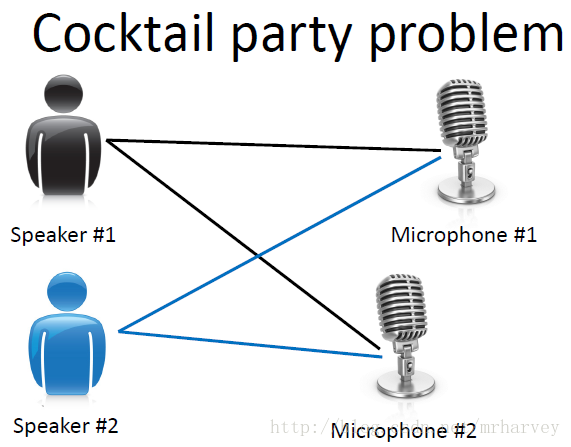
“鸡尾酒会问题”（cocktailparty problem）是在计算机语音识别领域的一个问题，当前语音识别技术已经可以以较高精度识别一个人所讲的话，但是当说话的人数为两人或者多人时，语音识别率就会极大的降低，这一难题被称为鸡尾酒会问题。

该问题描述的是给定混合信号，如何分离出鸡尾酒会中同时说话的每个人的独立信号。当有N个信号源时，通常假设观察信号也有N个（例如N个麦克风或者录音机）。该假设意味着混合矩阵是个方阵，即J = D，其中D是输入数据的维数，J是系统模型的维数。

 

要分离出鸡尾酒会中同时说话的每个人的独立信号，常用的方法是盲信号分离算法。

 

1 盲信号分离

1.1 简介

盲信号（BlindSource Separation，BSS）分离指的是从多个观测到的混合信号中分析出没有观测的原始信号。通常观测到的混合信号来自多个传感器的输出，并且传感器的输出信号独立性（线性不相关）。盲信号的“盲”字强调了两点：1)原始信号并不知道；2)对于信号混合的方法也不知道。

 

1.2 原理（简单的数学描述）

为了简单易懂，我们先看看只有两个信号源的情况，即观测信号也是只有两个。 和 是两个源信号； 和 是两个观测信号； 和 是对声源信号 和 的估计。矩阵A是混合矩阵（说得有点别扭，混合矩阵就是将两个信号混合在一起，然后产生输出两个观测信号）。W是权重矩阵（用于提取估计出声源信号）。下面就是BSS算法的主要流程图。

 

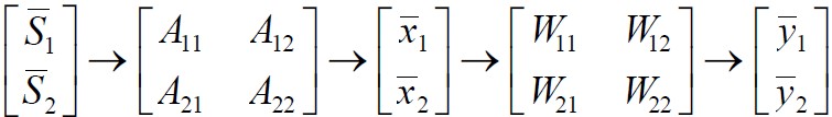
图1 BSS算法主要流程图

 

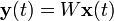
下面是图1所示流程的，矩阵表达形式：

 

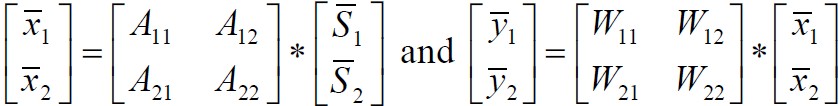
图2 BSS算法主要流程方程形式

 

 

看完简单的，我们看看难一点的，盲信号分离的模型。

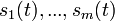
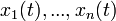
具有n个独立的信号源和n个独立的观察量,观察量和信号源具有如下的关系：

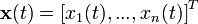
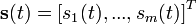
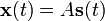
其中 , , A是一个的系数矩阵，原问题变成了已知和的独立性，求对 的估计问题。

假定有如下公式

其中是对 的估计，W是一个 系数矩阵，问题变成了如何有效的对矩阵W做出估计。

因此，BSS的主要工作是寻找一个线性滤波器或者是一个权重矩阵W。理想的条件下，W矩阵是A矩阵的逆矩阵。

由于参数空间不是欧几里得度量，在大多的情况下都是黎曼度量，因此对于W矩阵的求解选用自然梯度解法。

 

1.3 自然梯度法计算W矩阵

自然梯度法的计算公式为：

其中W为我们需要估计的矩阵。为步长,是一个非线性变换，比如

实际计算时y为一个矩阵，m为原始信号个数，k为采样点个数

 

计算步骤：

1)初始化W(0)为单位矩阵；

2)循环执行如下的步骤,直到W(n+1)与W(n)差异小于规定值(计算矩阵差异的方法可以人为规定)，有时候也人为规定迭代次数；

3)利用公式 ,(其中 )；

4)利用公式 ；

2 程序实现

1.main.m

% fftproject.m
% By: Johan Bylund（原始作者）
% 修改注释：Harvey
close all;
clear, clf, format compact;
% Makes a matrix out of wav files in project directory.
% The arreys will all be in the same length as the shortest one.
% Files longer than the shortest one will be truncated.
disp('Reading .wav files from project directory');
mic_1=wavread('000100100mix2.wav'); %Reading file from right microphone.
mic_2=wavread('000100100mix1.wav'); %Reading file from left microphone.
size(mic_1)
size(mic_2)

% The below operation makes them 1xN:
% 将矩阵设置成1*N的矩阵就一行多列的矩阵
mic_1=mic_1';
mic_2=mic_2';

% 规范长度，将长度统一在一起
if length(mic_1)>length(mic_2)
mic_1=mic_1(1:length(mic_2));
else
mic_2=mic_2(1:length(mic_1));
end
size(mic_1)
size(mic_2)
% 分别播放两个原始的接受源信号
disp('Playing the recording of the right microphone (closer to music)');
soundsc(mic_1)
disp('Playing the recording of the left microphone (closer to me)');
soundsc(mic_2)
subplot(2,1,1)
plot(mic_1), axis([0 16000 -0.12 0.12]);
title('Right microphone (closer to music)')
xlabel('Sampled points');
subplot(2,1,2)
plot(mic_2), axis([0 16000 -0.12 0.12]);
title('Left microphone (closer to me)')
xlabel('Sampled points');

% I also choose to look at the frequency spectra of the signal:
% 信号频谱经过快速傅立叶变换显示
Fs=8000; % Sampling frequency
% Matrix with the frequency spectra from the two microphones:
fftsounds=[real(fft(mic_1,Fs));real(fft(mic_2,Fs))];
f=[1:Fs/2];
figure(2)
subplot(2,1,1)
plot(f,fftsounds(1,f)), axis([0 4000 -15 15]);
title('Frequency spectra of the right microphone')
xlabel('Frequency (Hz)');
subplot(2,1,2)
plot(f,fftsounds(2,f)), axis([0 4000 -15 15]);
title('Frequency spectra of the left microphone')
xlabel('Frequency (Hz)');
% At first I tried the algorithm in the time domain, and it didn't
% manage to separate the two sources very well.
% After that I used the frequency spectra of the two microphone signals
% in the algorithm and it worked out much better.
% 算法开始了……
% 按照原作者说的话，使用频域来运算的效果会比时域要好（请看上面的英文注释）
sounds=[real(fft(mic_1));real(fft(mic_2))];
% N="number of microphones"
% P="number of points"
[N,P]=size(sounds) % P=?, N=2, in this case.
permute=randperm(P); % Generate a permutation vector.
s=sounds(:,permute); % Time-scrambled inputs for stationarity.
x=s;
mixes=sounds;
% Spheres the data (normalisation).
mx=mean(mixes');
c=cov(mixes');
x=x-mx'*ones(1,P); % Subtract means from mixes.
wz=2*inv(sqrtm(c)); % Get decorrelating matrix.
x=wz*x; % Decorrelate mixes so cov(x')=4*eye(N);
w=pi^2*rand(N); % Initialise unmixing matrix.
M=size(w,2); % M=N usually
sweep=0; oldw=w; olddelta=ones(1,N*N);
Id=eye(M);
% L="learning rate, B="points per block"
% Both are used in sep.m, which goes through the mixed signals
% in batch blocks of size B, adjusting weights, w, at the end
% of each block.
%L=0.01; B=30; sep
%L=0.001; B=30; sep % Annealing will improve solution.
%L=0.0001; B=30; sep % ...and so on
%for multiple sweeps:
L=0.0001; B=30;
for I=1:100
sep; % For details see sep.m
end;
uu=w*wz*mixes; % make unmixed sources
% Plot the two separated vectors in the frequency domain.
figure(3)
subplot(2,1,1)
plot(f,uu(1,f)), axis([0 4000 -22 22]);
title('Frequency spectra of one of the separated signals')
xlabel('Frequency (Hz)');
subplot(2,1,2)
plot(f,uu(2,f)), axis([0 4000 -22 22]);
title('Frequency spectra of the other separated signal')
xlabel('Frequency (Hz)');
% Transform signals back to time domain.
uu(2,:)=real(ifft(uu(2,:)));
uu(1,:)=real(ifft(uu(1,:)));
disp('Playing the first of the separated vectors');
soundsc(uu(1,:))
% Plot the vector that is played above.
figure(4);
subplot(2,1,1)
plot(uu(1,:)), axis([0 16000 -0.12 0.12]);
title('Plot of one of the separated vectors (time domain)')
disp('Playing the second of the separated vectors');
soundsc(uu(2,:))
% Plot the vector that is played above.
subplot(2,1,2)
plot(uu(2,:)), axis([0 16000 -0.12 0.12]);
title('Plot of the other separated vector (time domain)')

2. sep.m

% SEP goes once through the scrambled mixed speech signals, x 
% (which is of length P), in batch blocks of size B, adjusting weights,
% w, at the end of each block.
%
% I suggest a learning rate L, of 0.01 at least for 2->2 separation.
% But this will be unstable for higher dimensional data. Test it.
% Use smaller values. After convergence at a value for L, lower
% L and it will fine tune the solution.
%
% NOTE: this rule is the rule in our NC paper, but multiplied by w^T*w,
% as proposed by Amari, Cichocki & Yang at NIPS '95. This `natural
% gradient' method speeds convergence and avoids the matrix inverse in the 
% learning rule.

sweep=sweep+1; t=1;
noblocks=fix(P/B);
BI=B*Id;
for t=t:B:t-1+noblocks*B,
  u=w*x(:,t:t+B-1); 
  w=w+L*(BI+(1-2*(1./(1+exp(-u))))*u')*w;
end;
sepout

3. sepout.m

% SEPOUT - put whatever textual output report you want here.
%  Called after each pass through the data.
%  If your data is real, not artificially mixed, you will need
%  to comment out line 4, since you have no idea what the matrix 'a' is.
% 
[change,olddelta,angle]=wchange(oldw,w,olddelta); 
oldw=w;
fprintf('****sweep=%d, change=%.4f angle=%.1f deg., [N%d,M%d,P%d,B%d,L%.5f] \n',...
   sweep,change,180*angle/pi,N,M,P,B,L);
% w*wz*a     %should be a permutation matrix for artif. mixed data

上述代码中所使用的声音文件可以到这个网址下下载：http://research.ics.aalto.fi/ica/cocktail/cocktail_en.cgi

参考文献

[1]维基百科. 独立成分分析. http://zh.wikipedia.org/wiki/%E7%8B%AC%E7%AB%8B%E6%88%90%E5%88%86%E5%88%86%E6%9E%90,2014-1-14.

[2] 我爱公开课. Coursera公开课笔记: 斯坦福大学机器学习第一课“引言(Introduction)”. http://52opencourse.com/54/coursera%E5%85%AC%E5%BC%80%E8%AF%BE%E7%AC%94%E8%AE%B0-%E6%96%AF%E5%9D%A6%E7%A6%8F%E5%A4%A7%E5%AD%A6%E6%9C%BA%E5%99%A8%E5%AD%A6%E4%B9%A0%E7%AC%AC%E4%B8%80%E8%AF%BE-%E5%BC%95%E8%A8%80-introduction,2014-1-14.

[3]维基百科. 盲信号分离. http://zh.wikipedia.org/wiki/%E7%9B%B2%E4%BF%A1%E5%8F%B7%E5%88%86%E7%A6%BB,2014-1-14.

[4]Johan Bylund. A hunble attempt to solvethe “Cocktail-party” problem Using Blind Source Separation[EB].http://www.vislab.uq.edu.au/education/sc3/2001/johan/johan.pdf.