原文链接:

https://www.dailydoseofds.com/a-crash-course-on-building-rag-systems-part-1-with-implementations/

https://www.dailydoseofds.com/a-crash-course-on-building-rag-systems-part-2-with-implementations/

Introduction

We have also talked about vector databases, which are not new, but they have become heavily prevalent lately in the GenAI era, primarily due to their practical utility not just in LLMs but in other applications as well.

More specifically, vector databases come in handy in building RAG applications, which is a technique that combines the strengths of large language models (LLMs) with external knowledge sources.

This is depicted below.

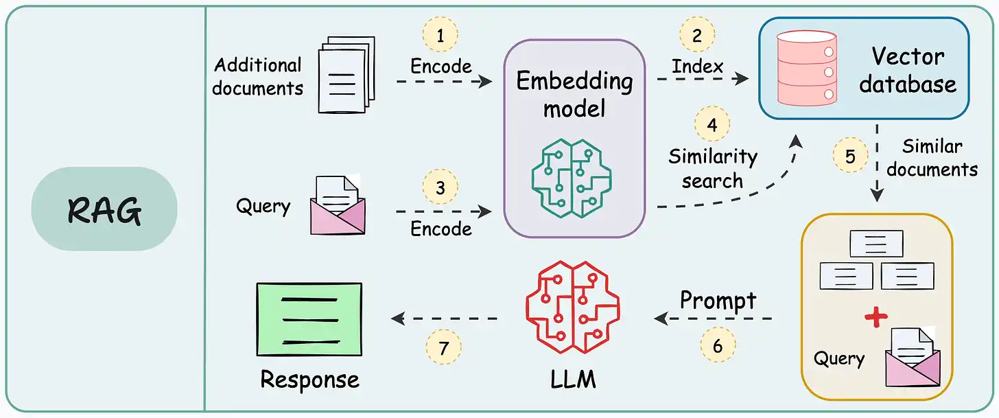
A typical RAG setup

The objective of this crash course is to help you implement these RAG systems from scratch using frameworks like Qdrant, Llama index, and Ollama.

Of course, if you don't know of these frameworks, don't worry, since that is what we intend to cover today with proper context, like we always do.

This comprehensive crash course will go into the depths of RAG by understanding its necessity and then cover a hands-on approach to building your own RAG system.

By the end of this article, you'll have a solid understanding of RAG and how to use it in your own applications.

Let's begin!

---

Recap on vector databases

Feel free to skip this section if you already know about them or have read the  deep dive on vector databases before.

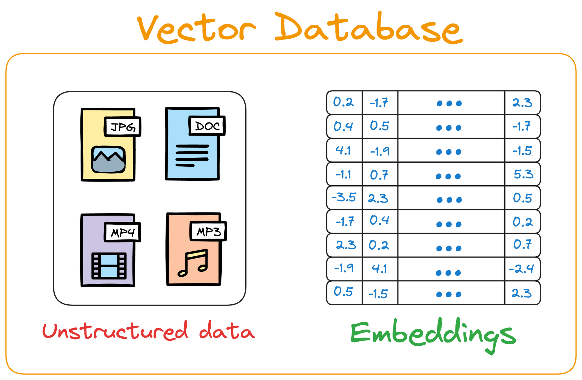
What are vector databases?

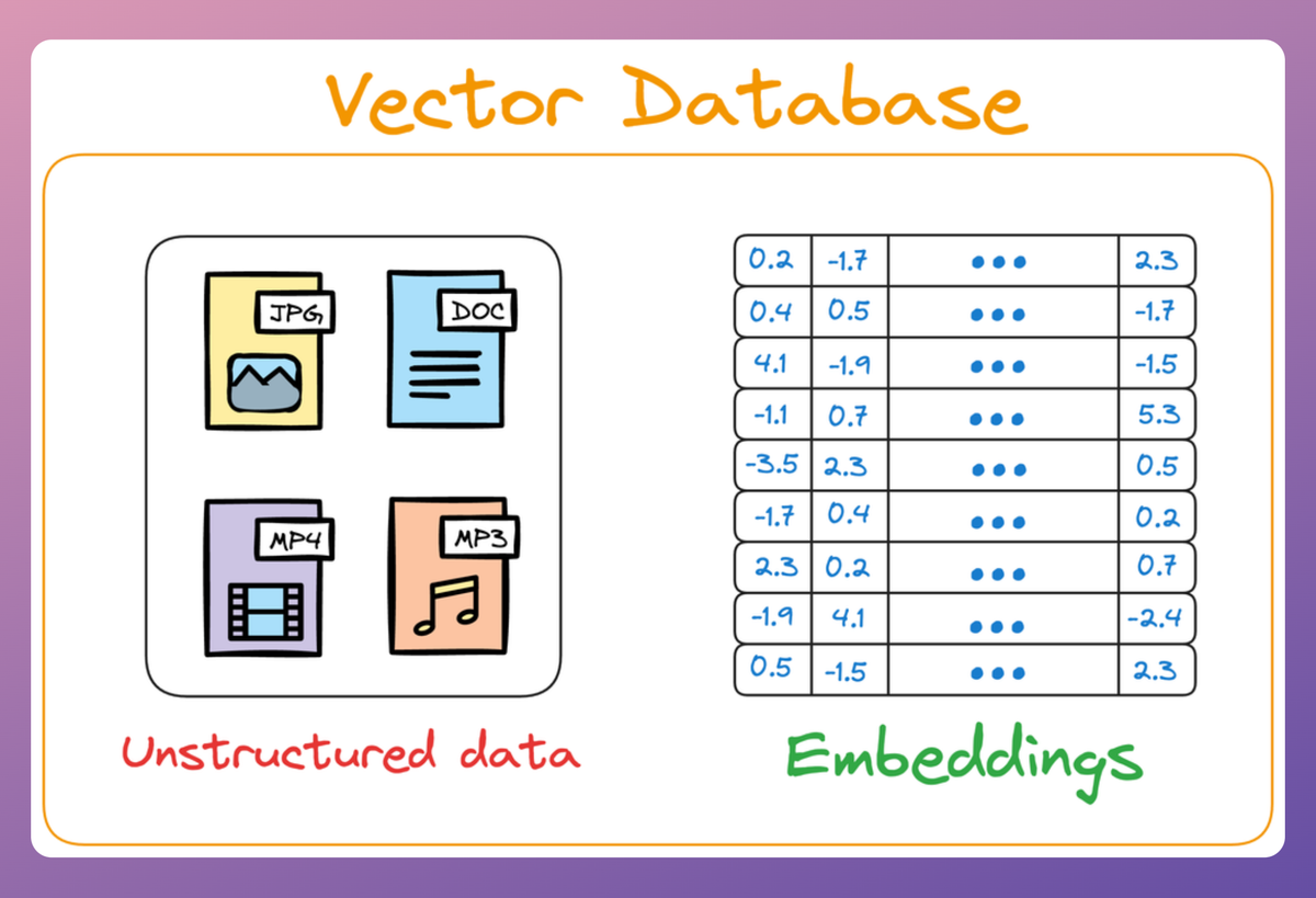
Simply put, a vector database stores unstructured data (text, images, audio, video, etc.) in the form of vector embeddings.

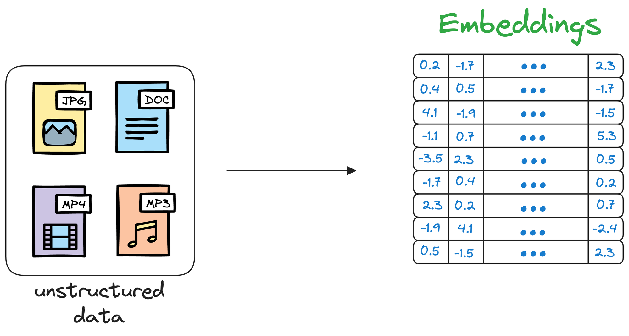
Each data point, whether a word, a document, an image, or any other entity, is transformed into a numerical vector using ML techniques (which we shall see ahead).

This numerical vector is called an embedding, and the model is trained in such a way that these vectors capture the essential features and characteristics of the underlying data.

Considering word embeddings, for instance, we may discover that in the embedding space, the embeddings of fruits are found close to each other, which cities form another cluster, and so on.

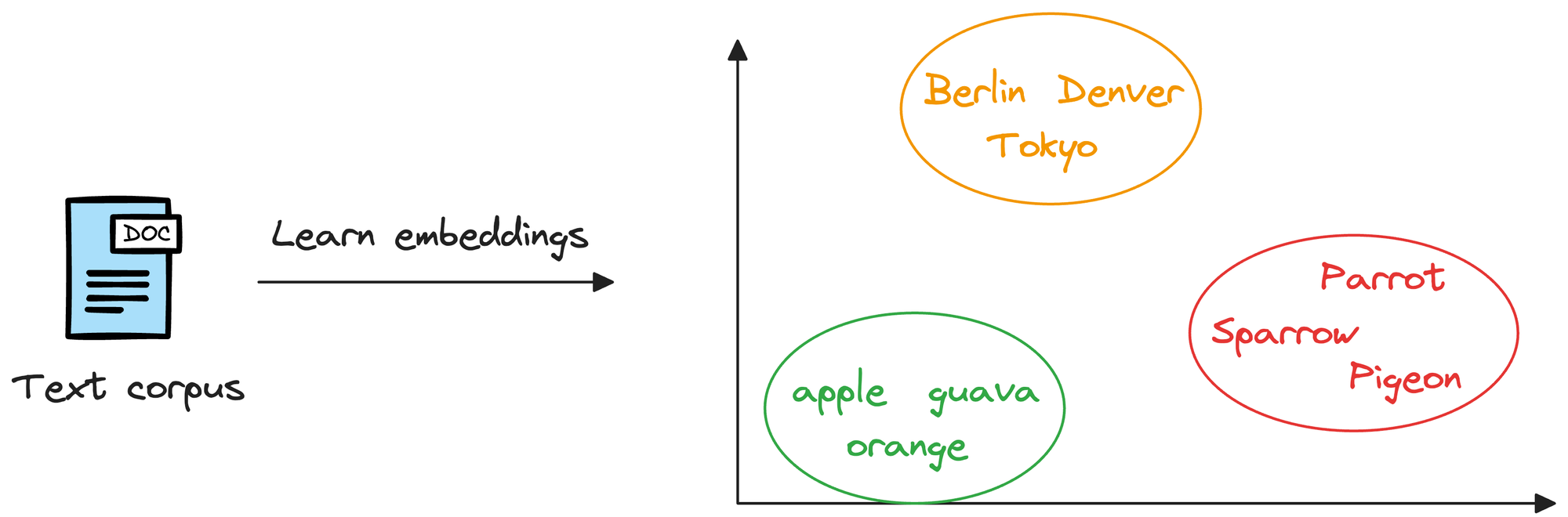
This shows that embeddings can learn the semantic characteristics of entities they represent (provided they are trained appropriately).

Once stored in a vector database, we can retrieve original objects that are similar to the query we wish to run on our unstructured data.

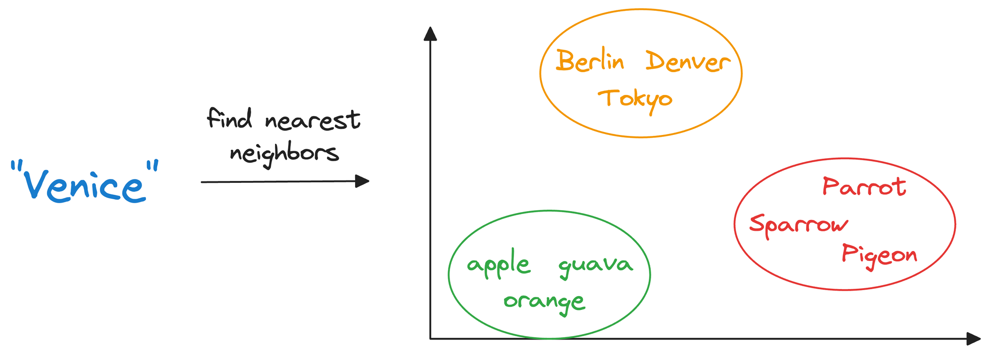
In other words, encoding unstructured data allows us to run many sophisticated operations like similarity search, clustering, and classification over it, which otherwise is difficult with traditional databases.

💡

To exemplify, when an e-commerce website provides recommendations for similar items or searches for a product based on the input query, we’re (in most cases) interacting with vector databases behind the scenes.

The purpose of vector databases

Let's imagine we have a collection of photographs from various vacations we’ve taken over the years. Each photo captures different scenes, such as beaches, mountains, cities, and forests.

Now, we want to organize these photos in a way that makes it easier to find similar ones quickly.

Traditionally, we might organize them by the date they were taken or the location where they were shot.

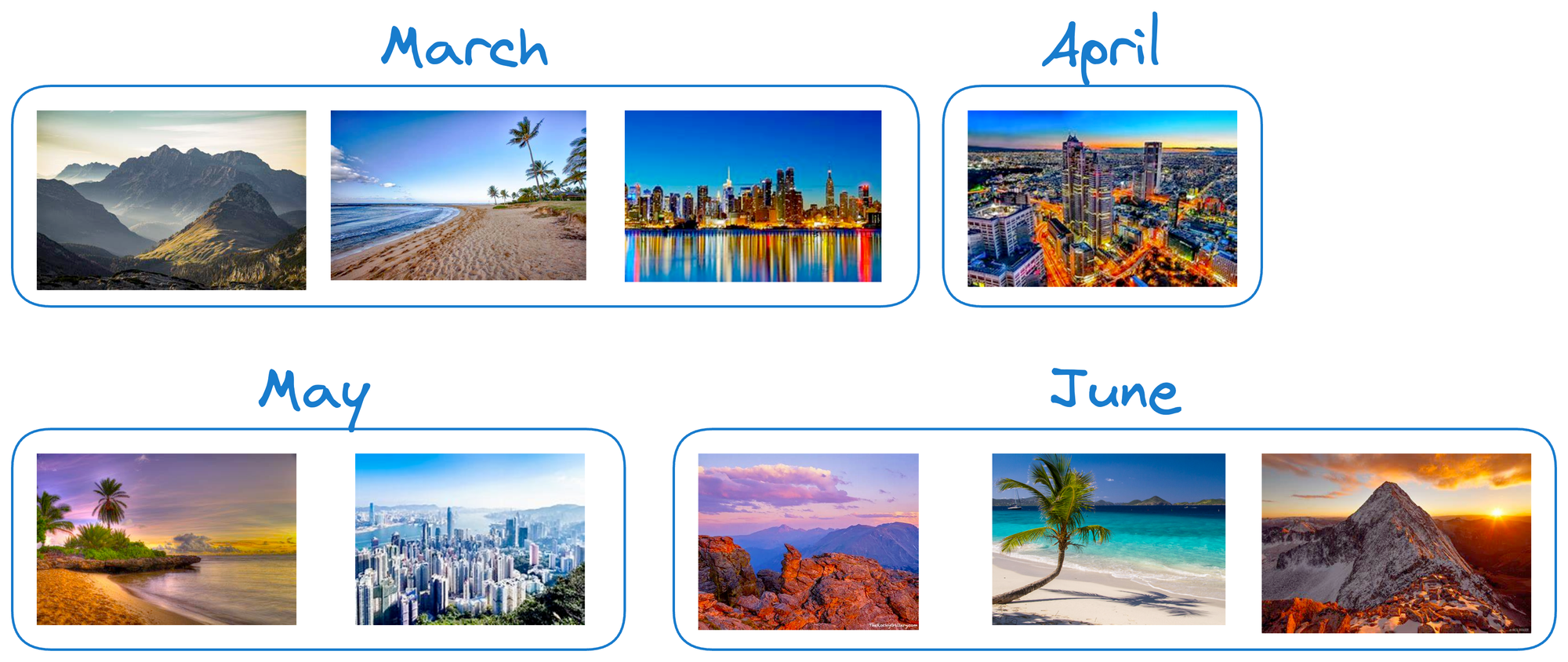
However, we can take a more sophisticated approach by encoding them as vectors.

More specifically, instead of relying solely on dates or locations, we could represent each photo as a set of numerical vectors that capture the essence of the image.

💡

While Google Photos doesn't explicitly disclose the exact technical details of its backend systems, I speculate that it uses a vector database to facilitate its image search and organization features, which you may have already used many times.

Let’s say we use an algorithm that converts each photo into a vector based on its color composition, prominent shapes, textures, people, etc.

Each photo is now represented as a point in a multi-dimensional space, where the dimensions correspond to different visual features and elements in the image.

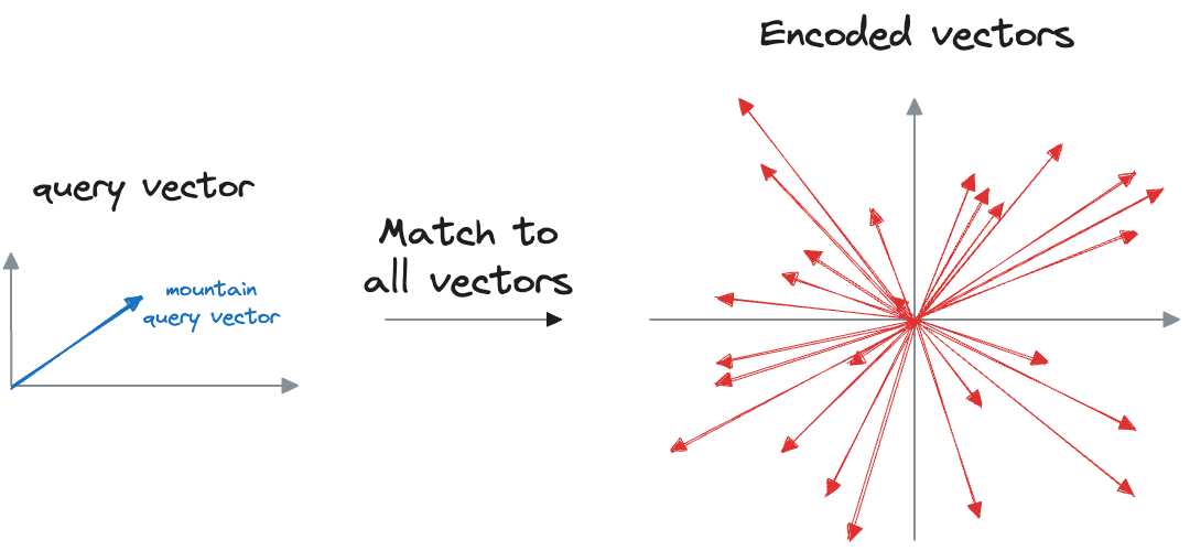
Now, when we want to find similar photos, say, based on our input text query, we encode the text query into a vector and compare it with image vectors.

Photos that match the query are expected to have vectors that are close together in this multi-dimensional space.

Suppose we wish to find images of mountains.

Since a vector maintains both the embeddings and the raw data that generated those embeddings, we can quickly find such photos by querying the vector database for images close to the vector representing the input query.

Simple, isn't it?

Of course, since a vector database can have millions of vectors, a traditional nearest neighbor search isn't feasible since it will measure the similarity with all vectors.

That is why we need approximate nearest neighbor (ANN) search algorithms.

The core idea is to narrow down the search space for the query vector, thereby improving the run-time performance.

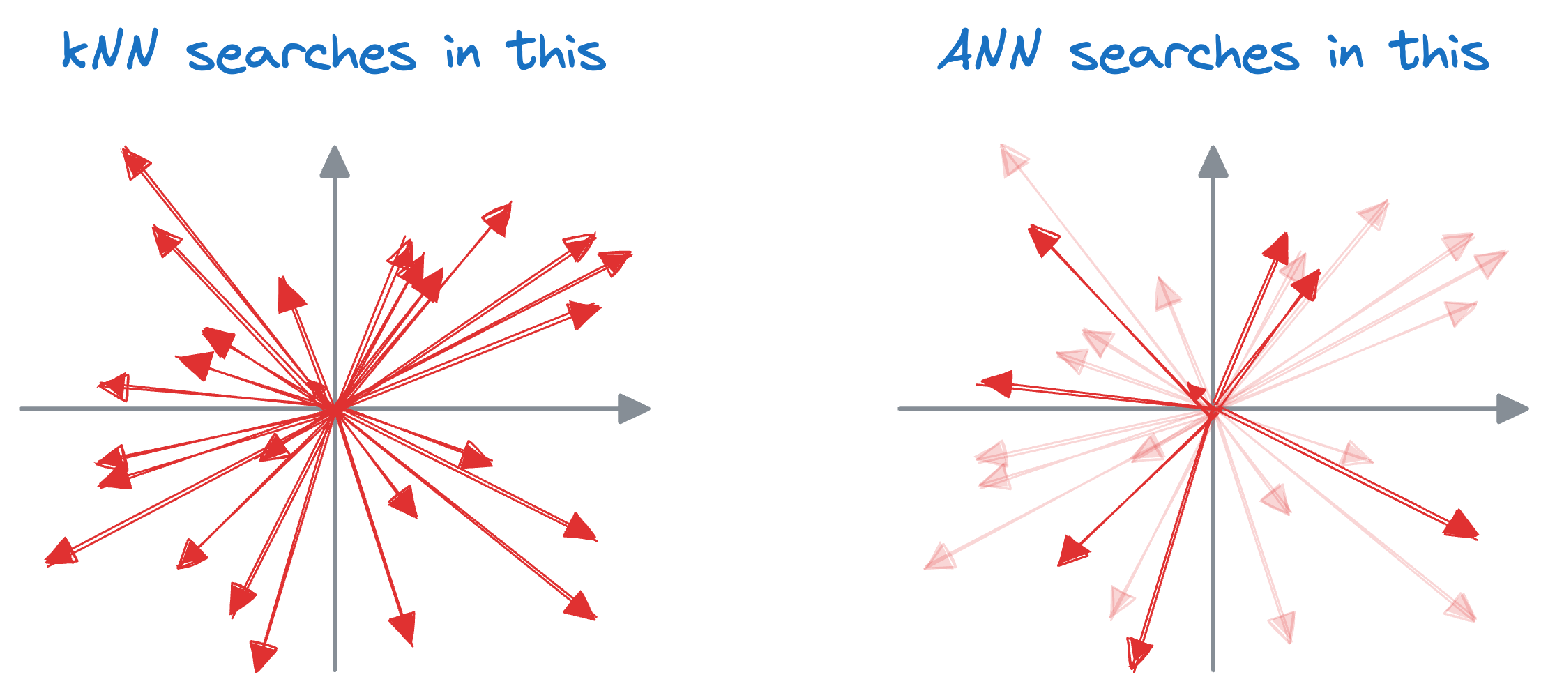
While they usually sacrifice a certain degree of precision compared to exact nearest neighbor methods, they offer significant performance gains, particularly in scenarios where real-time or near-real-time responses are required.

We discussed several ANN algorithms below:

A Beginner-friendly and Comprehensive Deep Dive on Vector Databases

Understanding every little detail on vector databases and their utility in LLMs, along with a hands-on demo.

​编辑Daily Dose of Data ScienceAvi Chawla

The purpose of vector databases in RAG

At this point, one interesting thing to learn is how exactly LLMs take advantage of vector databases.

In my experience, the biggest confusion that people typically face is:

Once we have trained our LLM, it will have some model weights for text generation. Where do vector databases fit in here?

Let's understand this.

To begin, we must understand that an LLM is deployed after learning from a static version of the corpus it was fed during training.

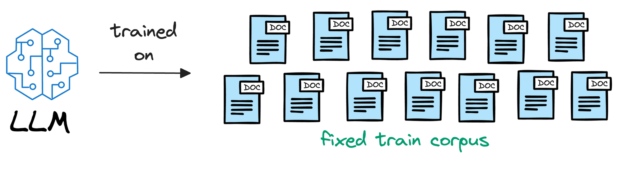
For instance, if the model was deployed after considering the data until 31st Jan 2024, and we use it, say, a week after training, it will have no clue about what happened in those days.

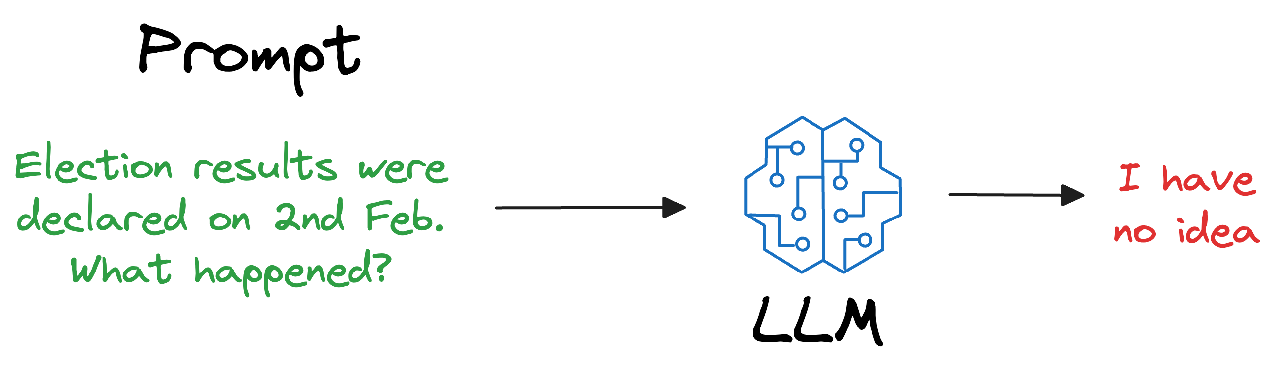
Repeatedly training a new model (or adapting the latest version) every single day on new data is impractical and cost-ineffective. In fact, LLMs can take weeks to train.

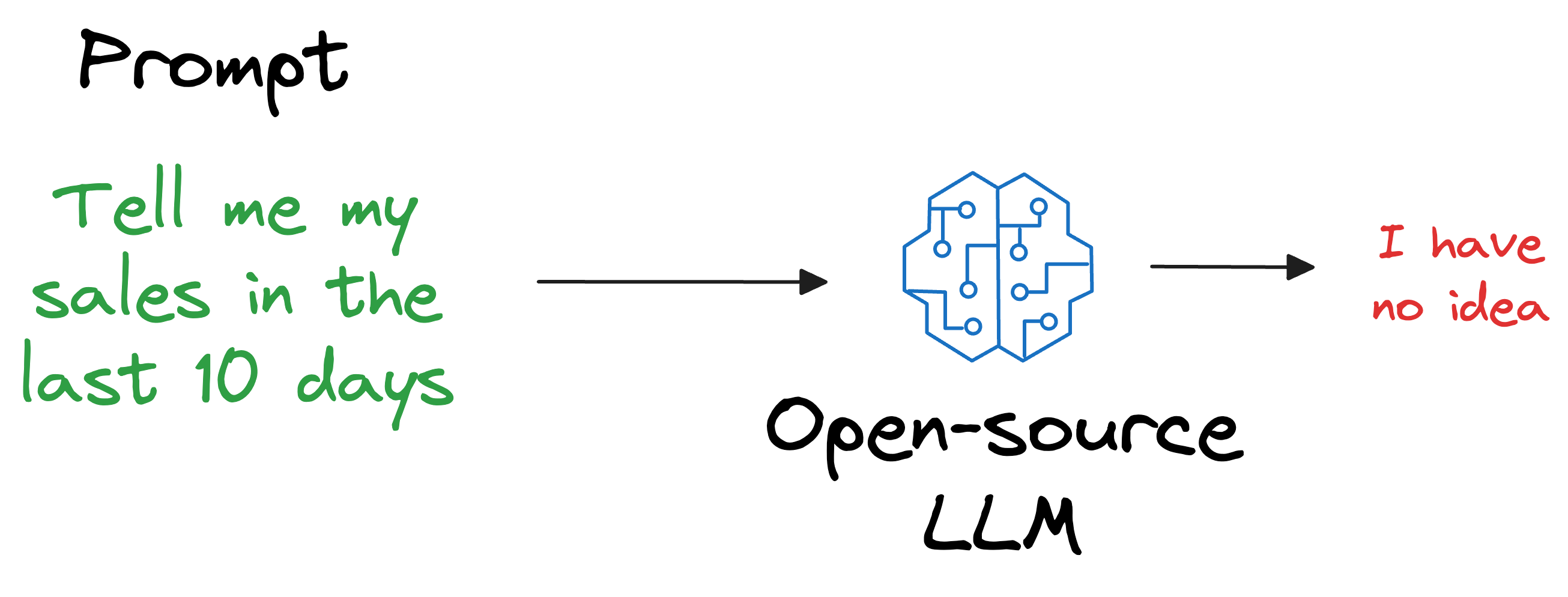
Also, what if we open-sourced the LLM and someone else wants to use it on their privately held dataset, which, of course, was not shown during training?

As expected, the LLM will have no clue about it.

But if you think about it, is it really our objective to train an LLM to know every single thing in the world?

Not at all!

That’s not our objective.

Instead, it is more about helping the LLM learn the overall structure of the language, and how to understand and generate it.

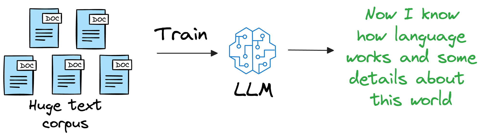
So, once we have trained this model on a ridiculously large enough training corpus, it can be expected that the model will have a decent level of language understanding and generation capabilities.

Thus, if we could figure out a way for LLMs to look up new information they were not trained on and use it in text generation (without training the model again), that would be great!

One way could be to provide that information in the prompt itself.

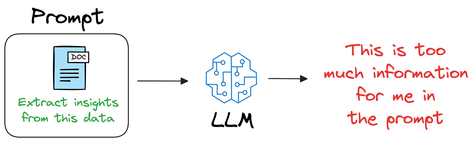
But since LLMs usually have a limit on the context window (number of words/tokens they can accept), the additional information can exceed that limit.

Vector databases solve this problem.

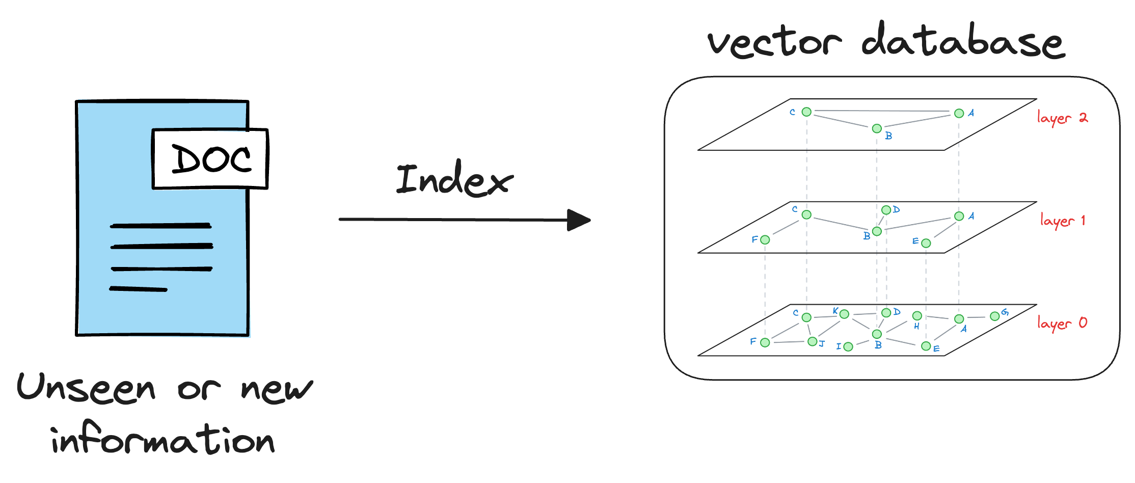
As discussed earlier in the article, vector databases store information in the form of vectors, where each vector captures semantic information about the piece of text being encoded.

Thus, we can maintain our available information in a vector database by encoding it into vectors using an embedding model.

When the LLM needs to access this information, it can query the vector database using an approximate similarity search with the prompt vector to find content that is similar to the input query vector.

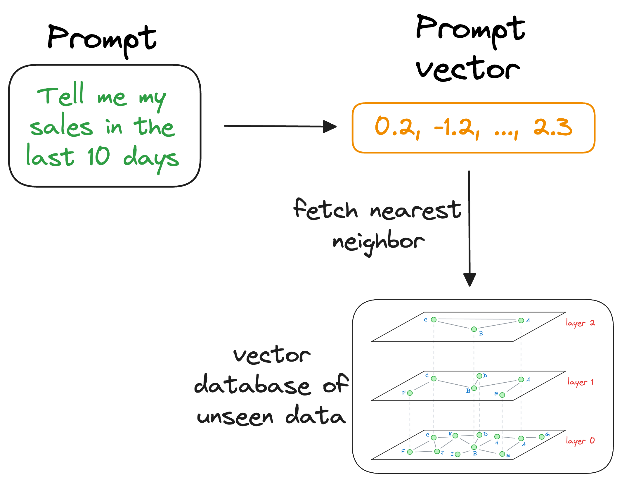
Once the approximate nearest neighbors have been retrieved, we gather the context corresponding to those specific vectors, which were stored at the time of indexing the data in the vector database (this raw data is stored as payload, which we will learn during implementation).

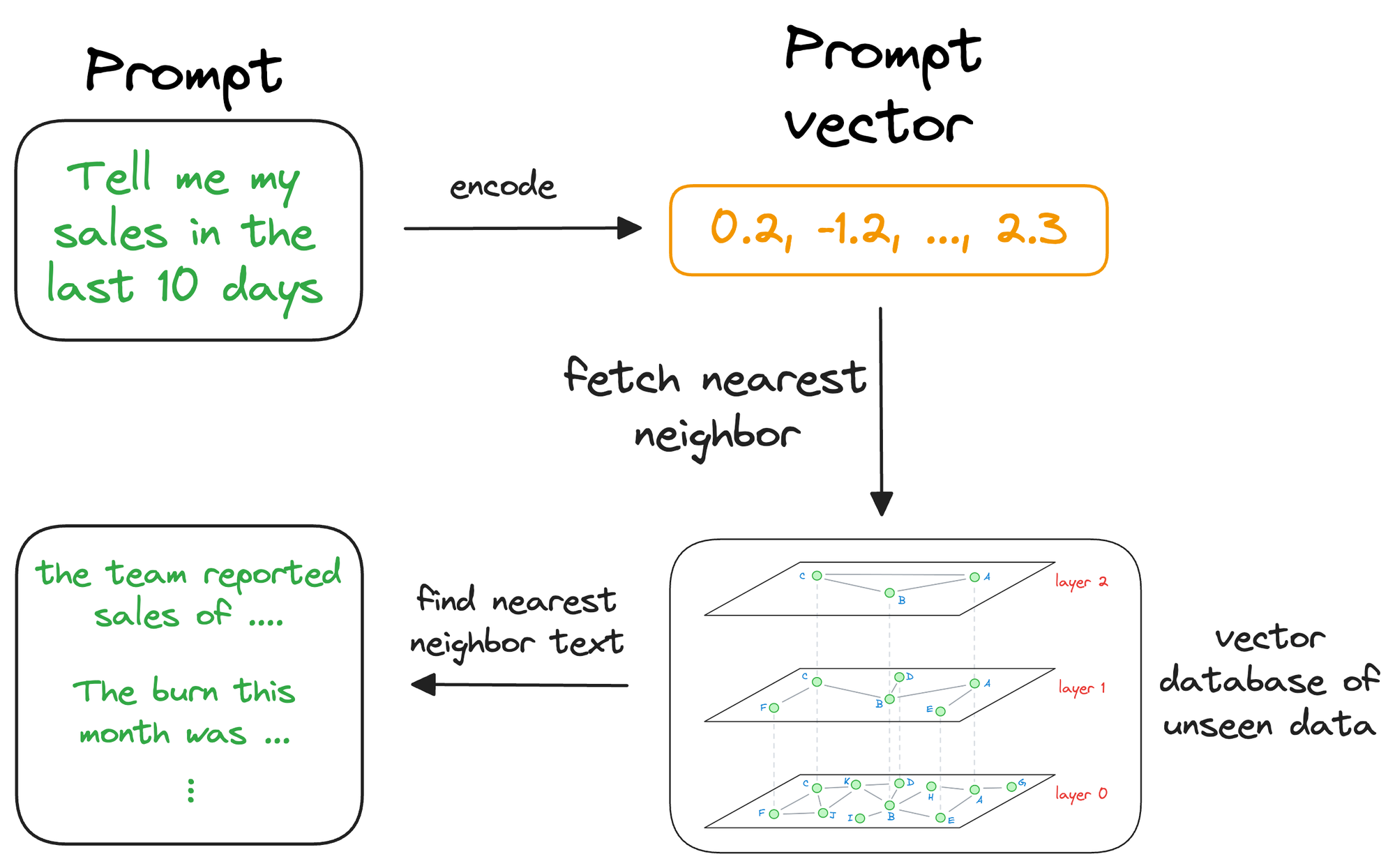
The above search process retrieves context that is similar to the query vector, which represents the context or topic the LLM is interested in.

We can augment this retrieved content along with the actual prompt provided by the user and give it as input to the LLM.

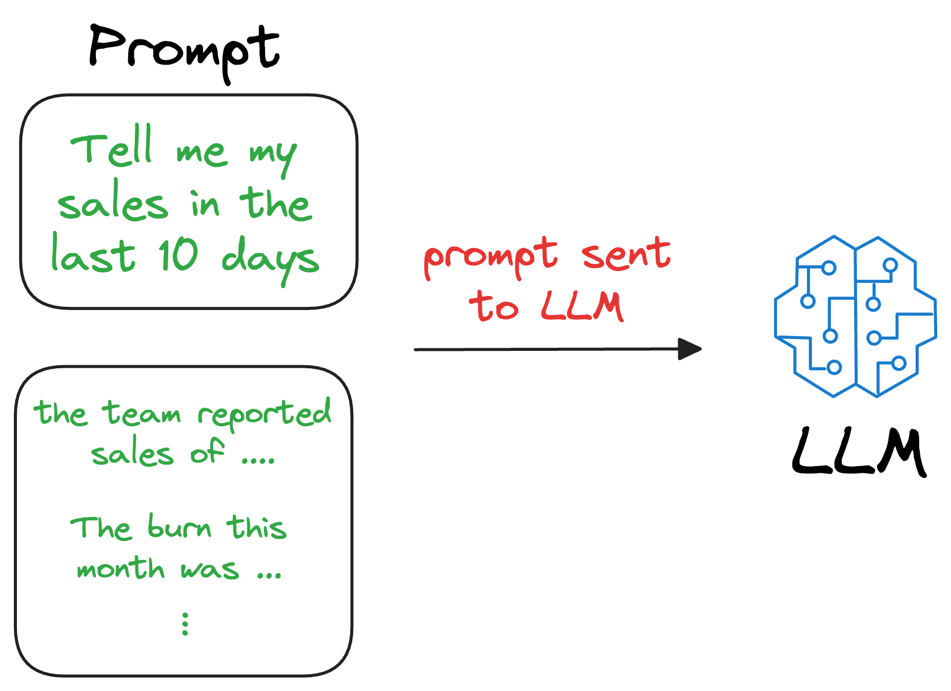
Consequently, the LLM can easily incorporate this info while generating text because it now has the relevant details available in the prompt.

And this is called Retrieval-Augmented Generation (RAG), which is explained below:

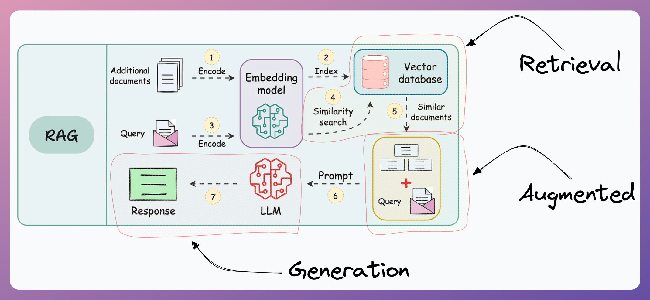
• Retrieval: Accessing and retrieving information from a knowledge source, such as a database or memory.
• Augmented: Enhancing or enriching something, in this case, the text generation process, with additional information or context.
• Generation: The process of creating or producing something, in this context, generating text or language.

With RAG, the language model can use the retrieved information (which is expected to be reliable) from the vector database to ensure that its responses are grounded in real-world knowledge and context, reducing the likelihood of hallucinations.

This makes the model's responses more accurate, reliable, and contextually relevant, while also ensuring that we don't have to train the LLM repeatedly on new data. This makes the model more "real-time" in its responses.

Now that we understand the purpose, let's get into the technical details.

---

Workflow of a RAG system

To build a RAG system, it's crucial to understand the foundational components that go into it and how they interact. Thus, in this section, let's explore each element in detail.

Here's an architecture diagram of a typical RAG setup:

Let's break it down step by step.

We start with some external knowledge that wasn't seen during training, and we want to augment the LLM with:

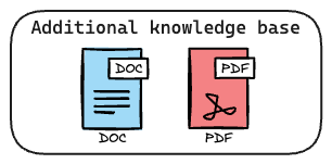
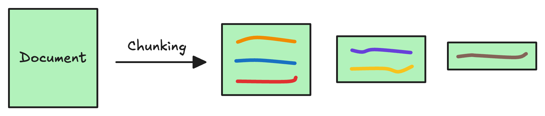
1) Create chunks

The first step is to break down this additional knowledge into chunks before embedding and storing it in the vector database.

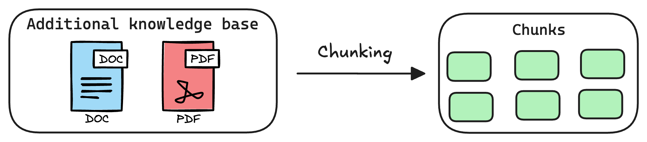
We do this because the additional document(s) can be pretty large. Thus, it is important to ensure that the text fits the input size of the embedding model.

Moreover, if we don't chunk, the entire document will have a single embedding, which won't be of any practical use to retrieve relevant context.

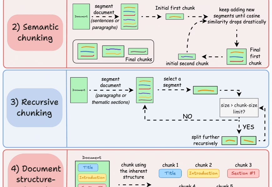
We covered chunking strategies recently in the newsletter here:

5 Chunking Strategies For RAG

...explained in a single frame.

​编辑Daily Dose of Data ScienceAvi Chawla

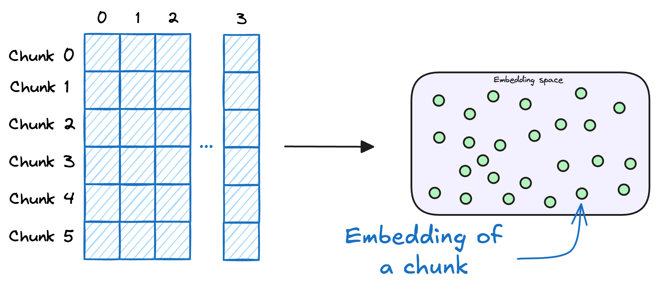
2) Generate embeddings

After chunking, we embed the chunks using an embedding model.

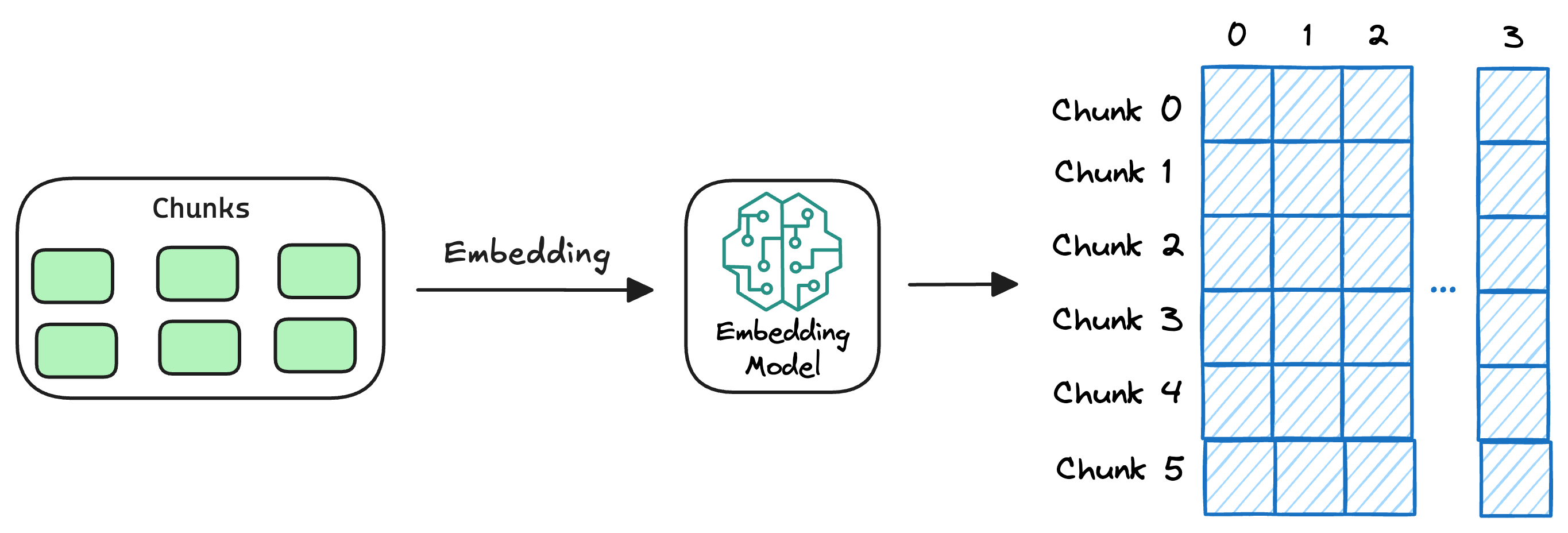
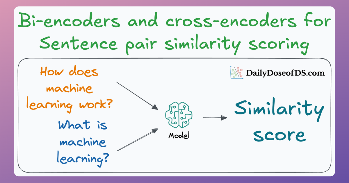
Since these are “context embedding models” (not word embedding models), models like bi-encoders (which we discussed last time) are highly relevant here.

Bi-encoders and Cross-encoders for Sentence Pair Similarity Scoring – Part 1

A deep dive into why BERT isn’t effective for sentence similarity and advancements that shaped this task forever.

​编辑Daily Dose of Data ScienceAvi Chawla

3) Store embeddings in a vector database

These embeddings are then stored in the vector database:

This shows that a vector database acts as a memory for your RAG application since this is precisely where we store all the additional knowledge, using which, the user's query will be answered.

💡

A vector database also stores the metadata and original content along with the vector embeddings.

With that, our vector databases has been created and information has been added. More information can be added to this if needed.

Now, we move to the query step.

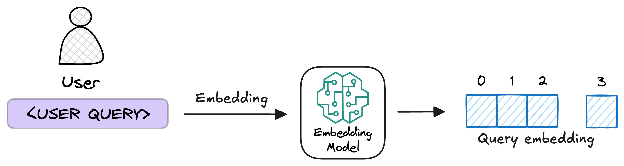
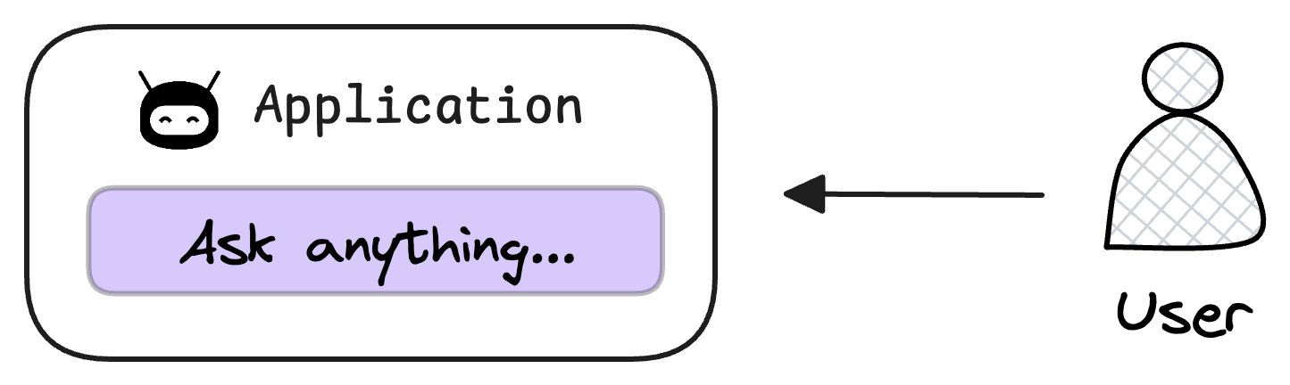
4) User input query

Next, the user inputs a query, a string representing the information they're seeking.

5) Embed the query

This query is transformed into a vector using the same embedding model we used to embed the chunks earlier in Step 2.

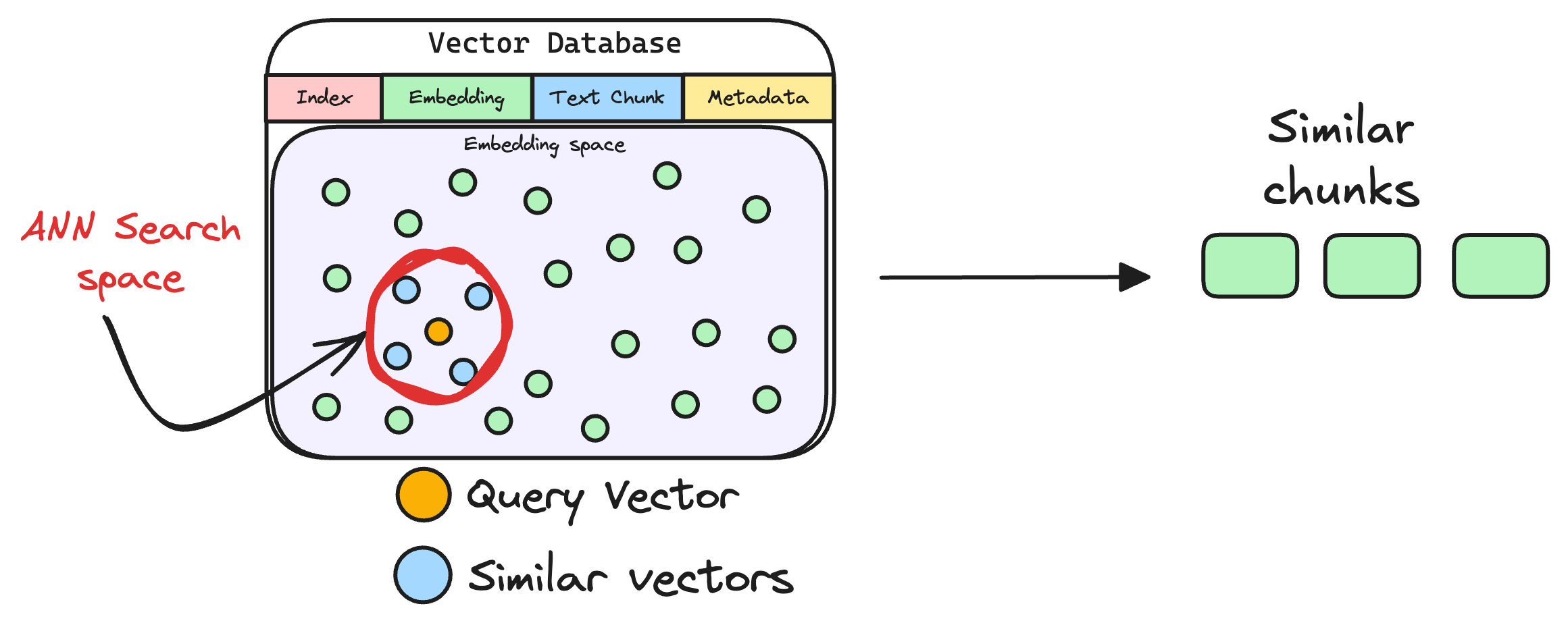
6) Retrieve similar chunks

The vectorized query is then compared against our existing vectors in the database to find the most similar information.

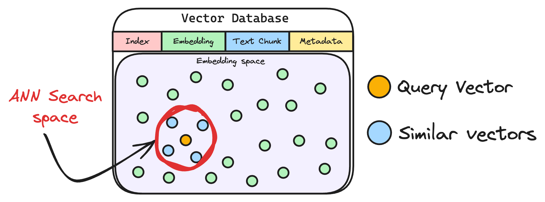
The vector database returns the k (a pre-defined parameter) most similar documents/chunks (using approximate nearest neighbor search).

It is expected that these retrieved documents contain information related to the query, providing a basis for the final response generation.

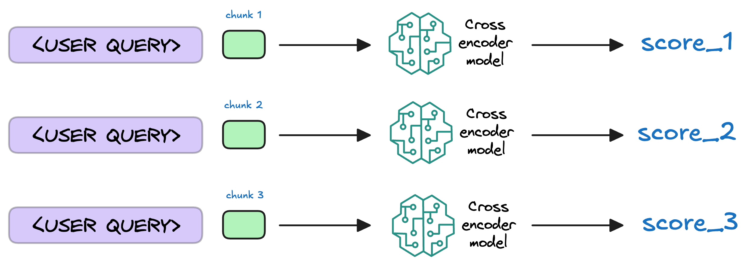
7) Re-rank the chunks

After retrieval, the selected chunks might need further refinement to ensure the most relevant information is prioritized.

In this re-ranking step, a more sophisticated model (often a cross-encoder, which we discussed last week) evaluates the initial list of retrieved chunks alongside the query to assign a relevance score to each chunk.

Introduction

In Part 1 of our RAG series, we explored the foundations of RAG, walking through each part and showing how they come together to create a powerful tool for information retrieval and synthesis.

But RAG (Retrieval-Augmented Generation) is not magic.

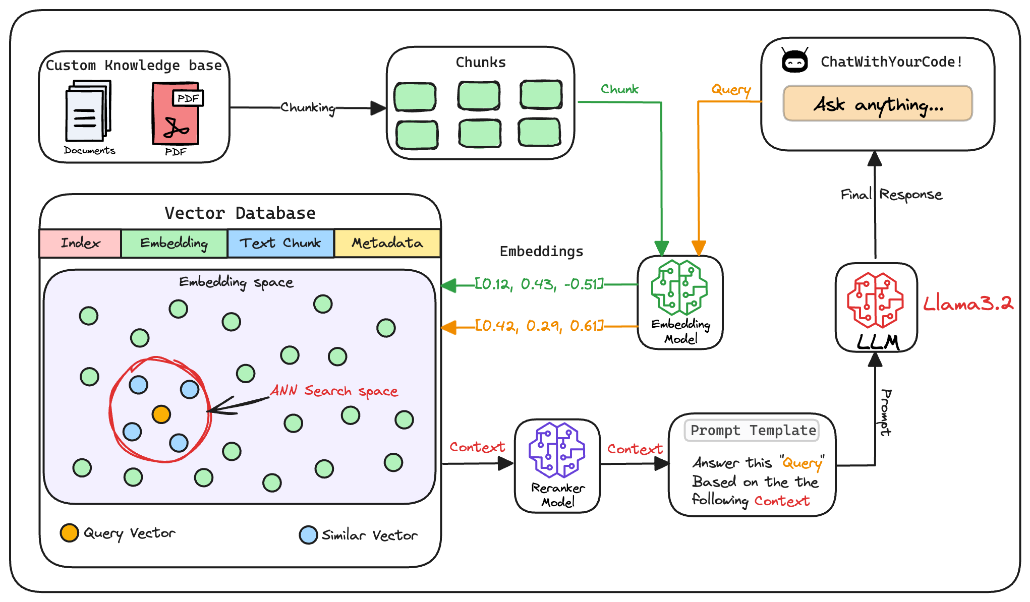
While it may feel like a seamless process involving inputting a question and receiving an accurate, contextually rich answer, a lot is happening under the hood, as depicted below:

As shown above, a RAG system relies on multiple interdependent components: a retrieval engine, a re-ranking model, and a generative model, each designed to perform a specific function.

Thus, while an end-to-end nicely integrated RAG system may seem like it “just works,” relying on them without thorough evaluation can be risky—especially if they’re powering applications where accuracy and context matter.

That is why, just like any other intelligence-driven system, RAG systems need evaluation as well since SO MANY things could go wrong in production:

• Chunking might not be precise and useful.
• The retrieval model might not always fetch the most relevant document.
• The generative model might misinterpret the context, leading to inaccurate or misleading answers.
• And more.

Part 2 (this article) of our RAG crash course is dedicated to the practicalities of RAG evaluation.

We’ll cover why it’s essential, the metrics that matter, and how to automate these evaluations, everything with implementations.

By the end, you’ll have a structured approach to assess your RAG system’s performance and maintain observability over its inner workings.

Make sure you have read Part 1 before proceeding with the RAG evaluation.

Nonetheless, we'll do a brief overview below for a quick recap.

Let's begin!

---

A quick recap

Feel free to skip section if you have already read Part 1 and move to the next section instead.

To build a RAG system, it's crucial to understand the foundational components that go into it and how they interact. Thus, in this section, let's explore each element in detail.

Here's an architecture diagram of a typical RAG setup:

Let's break it down step by step.

We start with some external knowledge that wasn't seen during training, and we want to augment the LLM with:

1) Create chunks

The first step is to break down this additional knowledge into chunks before embedding and storing it in the vector database.

We do this because the additional document(s) can be pretty large. Thus, it is important to ensure that the text fits the input size of the embedding model.

Moreover, if we don't chunk, the entire document will have a single embedding, which won't be of any practical use to retrieve relevant context.

We covered chunking strategies recently in the newsletter here:

5 Chunking Strategies For RAG

...explained in a single frame.

​编辑Daily Dose of Data ScienceAvi Chawla

2) Generate embeddings

After chunking, we embed the chunks using an embedding model.

Since these are “context embedding models” (not word embedding models), models like bi-encoders (which we discussed recently) are highly relevant here.

Bi-encoders and Cross-encoders for Sentence Pair Similarity Scoring – Part 1

A deep dive into why BERT isn’t effective for sentence similarity and advancements that shaped this task forever.

​编辑Daily Dose of Data ScienceAvi Chawla

3) Store embeddings in a vector database

These embeddings are then stored in the vector database:

This shows that a vector database acts as a memory for your RAG application since this is precisely where we store all the additional knowledge, using which the user's query will be answered.

💡

A vector database also stores the metadata and original content along with the vector embeddings.

With that, our vector databases has been created and information has been added. More information can be added to this if needed.

Now, we move to the query step.

4) User input query

Next, the user inputs a query, a string representing the information they're seeking.

5) Embed the query

This query is transformed into a vector using the same embedding model we used to embed the chunks earlier in Step 2.

6) Retrieve similar chunks

The vectorized query is then compared against our existing vectors in the database to find the most similar information.

The vector database returns the k (a pre-defined parameter) most similar documents/chunks (using approximate nearest neighbor search).

It is expected that these retrieved documents contain information related to the query, providing a basis for the final response generation.

7) Re-rank the chunks

After retrieval, the selected chunks might need further refinement to ensure the most relevant information is prioritized.

In this re-ranking step, a more sophisticated model (often a cross-encoder, which we discussed last week) evaluates the initial list of retrieved chunks alongside the query to assign a relevance score to each chunk.

This process rearranges the chunks so that the most relevant ones are prioritized for the response generation.

That said, not every RAG app implements this, and typically, they just rely on the similarity scores obtained in step 6 while retrieving the relevant context from the vector database.

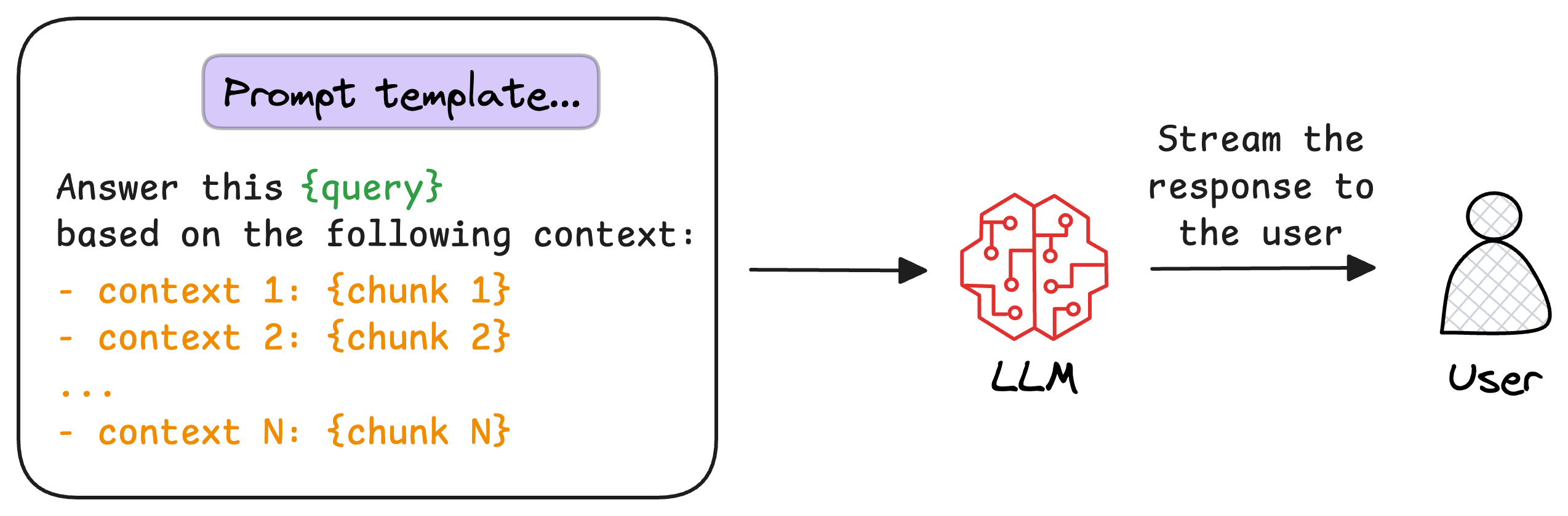
8) Generate the final response

Almost done!

Once the most relevant chunks are re-ranked, they are fed into the LLM.

This model combines the user's original query with the retrieved chunks in a prompt template to generate a response that synthesizes information from the selected documents.

This is depicted below:

---

Metrics for RAG evaluation

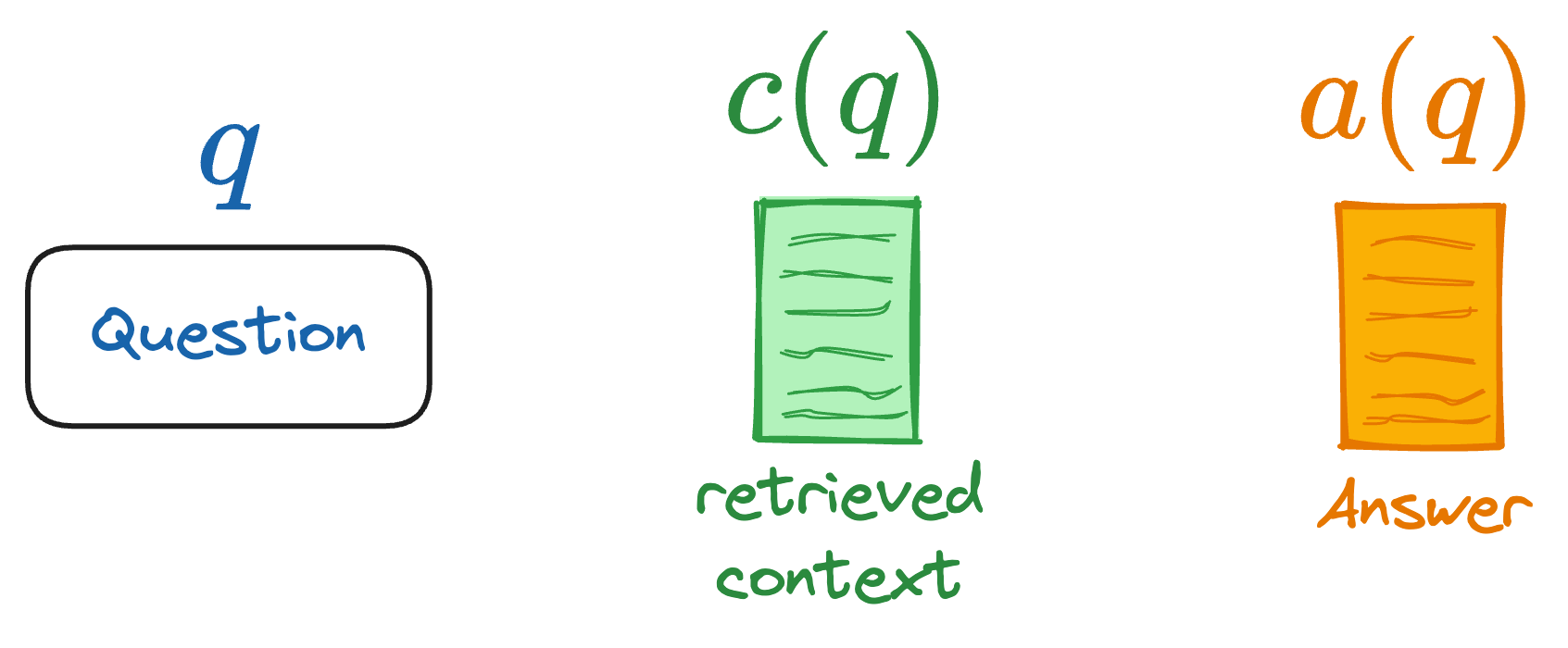
Typically, when evaluating a RAG system, we do not have access to human-annotated datasets or reference answers since the downstream application can be HIGHLY specific due to the capabilities of LLMs.

Therefore, we prefer self-contained or reference-free metrics that capture the “quality” of the generated response, which is precisely what matters in RAG applications.

For the discussion ahead, we'll consider these notations: