

Swin-Transformer网与源码
论文名称:Swin Transformer: Hierarchical Vision Transformer using Shifted Windows原论文地址: https://arxiv.org/abs/2103.14030官方开源代码地址:https://github.com/microsoft/Swin-TransformerPytorch实现代码: pytorch_classifica
论文名称:Swin Transformer: Hierarchical Vision Transformer using Shifted Windows
原论文地址: https://arxiv.org/abs/2103.14030
官方开源代码地址:https://github.com/microsoft/Swin-Transformer
Pytorch实现代码: pytorch_classification/swin_transformer
Tensorflow2实现代码:tensorflow_classification/swin_transformer
1 整体框架
首先来简单对比下Swin Transformer和之前的Vision Transformer。下图左边是Swin Transformer,右边是Vision Transformer结构。

通过对比至少可以看出两点不同:
- Swin Transformer使用了类似卷积神经网络中的层次化构建方法(Hierarchical feature maps),比如特征图尺寸中有对图像下采样4倍的,8倍的以及16倍的,这样的backbone有助于在此基础上构建目标检测,实例分割等任务。而在之前的Vision Transformer中是一开始就直接下采样16倍,后面的特征图也是维持这个下采样率不变。
- 在Swin Transformer中使用了Windows Multi-Head Self-Attention(W-MSA)的概念,比如在下图的4倍下采样和8倍下采样中,将特征图划分成了多个不相交的区域(Window),并且Multi-Head Self-Attention只在每个窗口(Window)内进行。相对于Vision Transformer中直接对整个(Global)特征图进行Multi-Head Self-Attention,这样做的目的是能够减少计算量的,尤其是在浅层特征图很大的时候。这样做虽然减少了计算量但也会隔绝不同窗口之间的信息传递,所以在论文中作者又提出了 Shifted Windows Multi-Head Self-Attention(SW-MSA)的概念,通过此方法能够让信息在相邻的窗口中进行传递,后面会细讲。
接下来,简单看下原论文中给出的关于Swin Transformer(Swin-T)网络的架构图。通过图(a)可以看出整个框架的基本流程如下:

- 首先将图片输入到Patch Partition模块中进行分块,即每4x4相邻的像素为一个Patch,然后在channel方向展平(flatten)。假设输入的是RGB三通道图片,那么每个patch就有4x4=16个像素,然后每个像素有R、G、B三个值所以展平后是16x3=48,所以通过Patch Partition后图像shape由 [H, W, 3]变成了 [H/4, W/4, 48]。然后在通过Linear Embeding层对每个像素的channel数据做线性变换,由48变成C,即图像shape再由 [H/4, W/4, 48]变成了 [H/4, W/4, C]。其实在源码中Patch Partition和Linear Embeding就是直接通过一个卷积层实现的,和之前Vision Transformer中讲的 Embedding层结构一模一样。
- 然后就是通过四个Stage构建不同大小的特征图,除了Stage1中先通过一个Linear Embeding层外,剩下三个stage都是先通过一个Patch Merging层进行下采样(后面会细讲)。然后都是重复堆叠Swin Transformer Block注意这里的Block其实有两种结构,如图(b)中所示,这两种结构的不同之处仅在于一个使用了W-MSA结构,一个使用了SW-MSA结构。而且这两个结构是成对使用的,先使用一个W-MSA结构再使用一个SW-MSA结构。所以你会发现堆叠Swin Transformer Block的次数都是偶数(因为成对使用)。
- 最后对于分类网络,后面还会接上一个Layer Norm层、全局池化层以及全连接层得到最终输出。图中没有画,但源码中是这样做的。
接下来,在分别对Patch Merging、W-MSA、SW-MSA以及使用到的相对位置偏执(relative position bias)进行详解。关于Swin Transformer Block中的MLP结构和Vision Transformer中的结构是一样的,所以这里也不在赘述,参考。
下面是Swin-Transformer主体源码:
源码:
class SwinTransformer(nn.Module):

    def __init__(self, img_size=224, patch_size=4, in_chans=3, num_classes=1000,
                 embed_dim=96, depths=[2, 2, 6, 2], num_heads=[3, 6, 12, 24],
                 window_size=7, mlp_ratio=4., qkv_bias=True, qk_scale=None,
                 drop_rate=0., attn_drop_rate=0., drop_path_rate=0.1,
                 norm_layer=nn.LayerNorm, ape=False, patch_norm=True,
                 use_checkpoint=False, **kwargs):
        super().__init__()

        self.num_classes = num_classes
        self.num_layers = len(depths)
        self.embed_dim = embed_dim
        self.ape = ape
        self.patch_norm = patch_norm
        self.num_features = int(embed_dim * 2 ** (self.num_layers - 1))
        self.mlp_ratio = mlp_ratio

        # split image into non-overlapping patches
        # 就是模型结构的 Patch Partition 图片变成 (B, H//4 * W//4, embed_dim)
        self.patch_embed = PatchEmbed(
            img_size=img_size, patch_size=patch_size, in_chans=in_chans, embed_dim=embed_dim,
            norm_layer=norm_layer if self.patch_norm else None)
        # 图像缩小4倍后的 patchers num
        num_patches = self.patch_embed.num_patches
        # 图像缩小4倍后的尺寸
        patches_resolution = self.patch_embed.patches_resolution
        self.patches_resolution = patches_resolution

        # absolute position embedding
        if self.ape:
            # 生成绝对位置编码 num_patches = H//4 * W//4 和经过PatchEmbed后的图片尺寸一致
            # 对应网络结构中的 linear embedding 网络结构
            self.absolute_pos_embed = nn.Parameter(torch.zeros(1, num_patches, embed_dim))
            # 绝对位置编码参数初始化
            trunc_normal_(self.absolute_pos_embed, std=.02)
        # 添加dropout
        self.pos_drop = nn.Dropout(p=drop_rate)

        # stochastic depth
        # 给网络层数每层设置随机dropout rate
        dpr = [x.item() for x in torch.linspace(0, drop_path_rate, sum(depths))]  # stochastic depth decay rule

        # build layers
        self.layers = nn.ModuleList()
        # 构建四层 w-msa 网络结构
        # input_resolution 表示每层会缩小 2**i_layer 倍 与给出的模型结构图展示的图像大小缩小倍数对应
        # depth block 深度
        # num_heads 多头数量
        # window_size 窗口大小
        # mlp_ratio Ratio of mlp hidden dim to embedding dim.
        # drop_path  dropout rate
        # downsample 下采样 前三个block 会进行下采样 第四个block 不会在进行下采样
        for i_layer in range(self.num_layers):
            layer = BasicLayer(dim=int(embed_dim * 2 ** i_layer),
                               input_resolution=(patches_resolution[0] // (2 ** i_layer),
                                                 patches_resolution[1] // (2 ** i_layer)),
                               depth=depths[i_layer],
                               num_heads=num_heads[i_layer],
                               window_size=window_size,
                               mlp_ratio=self.mlp_ratio,
                               qkv_bias=qkv_bias, qk_scale=qk_scale,
                               drop=drop_rate, attn_drop=attn_drop_rate,
                               drop_path=dpr[sum(depths[:i_layer]):sum(depths[:i_layer + 1])],
                               norm_layer=norm_layer,
                               downsample=PatchMerging if (i_layer < self.num_layers - 1) else None,
                               use_checkpoint=use_checkpoint)
            self.layers.append(layer)
        # 层归一化
        self.norm = norm_layer(self.num_features)
        # 平均池化
        self.avgpool = nn.AdaptiveAvgPool1d(1)
        # 网络输出
        self.head = nn.Linear(self.num_features, num_classes) if num_classes > 0 else nn.Identity()
        # 模型所以参数进行初始化
        self.apply(self._init_weights)

    def _init_weights(self, m):
        if isinstance(m, nn.Linear):
            trunc_normal_(m.weight, std=.02)
            if isinstance(m, nn.Linear) and m.bias is not None:
                nn.init.constant_(m.bias, 0)
        elif isinstance(m, nn.LayerNorm):
            nn.init.constant_(m.bias, 0)
            nn.init.constant_(m.weight, 1.0)

    @torch.jit.ignore
    def no_weight_decay(self):
        return {'absolute_pos_embed'}

    @torch.jit.ignore
    def no_weight_decay_keywords(self):
        return {'relative_position_bias_table'}

    def forward_features(self, x):
        # path_embed 就是模型结构的 Patch Partition 图片变成 (B, H//4 * W//4, embed_dim)
        x = self.patch_embed(x)
        # 是否使用绝对位置编码
        if self.ape:
            x = x + self.absolute_pos_embed
        x = self.pos_drop(x)
        # 经过4个 swin transformer block
        for layer in self.layers:
            x = layer(x)
        # 进行层归一化
        x = self.norm(x)  # B L C
        # 平局池化
        x = self.avgpool(x.transpose(1, 2))  # B C 1
        # 在第二个维度展平
        x = torch.flatten(x, 1)
        return x

    def forward(self, x):
        # 进行前向计算
        x = self.forward_features(x)
        # 模型最后输出用来进行分类 (b, c)
        x = self.head(x)
        return x

    def flops(self):
        """
        这个方法是用来计算模型性能的
        floating point operations per second
        """
        flops = 0
        flops += self.patch_embed.flops()
        for i, layer in enumerate(self.layers):
            flops += layer.flops()
        flops += self.num_features * self.patches_resolution[0] * self.patches_resolution[1] // (2 ** self.num_layers)
        flops += self.num_features * self.num_classes
        return flops
2 Patch Merging详解
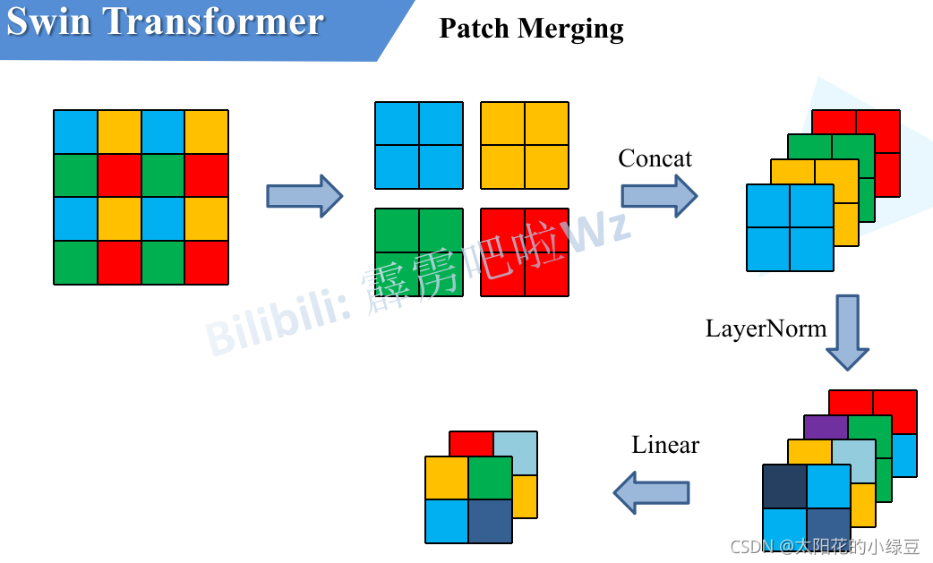
前面有说,在每个Stage中首先要通过一个Patch Merging层进行下采样(Stage1除外)。如下图所示,假设输入Patch Merging的是一个4x4大小的单通道特征图(feature map),Patch Merging会将每个2x2的相邻像素划分为一个patch,然后将每个patch中相同位置(同一颜色)像素给拼在一起就得到了4个feature map。接着将这四个feature map在深度方向进行concat拼接,然后在通过一个LayerNorm层。最后通过一个全连接层在feature map的深度方向做线性变化,将feature map的深度由C变成C/2。通过这个简单的例子可以看出,通过Patch Merging层后,feature map的高和宽会减半,深度会翻倍。
源码:
class PatchEmbed(nn.Module):

    def __init__(self, img_size=224, patch_size=4, in_chans=3, embed_dim=96, norm_layer=None):
        super().__init__()
        img_size = to_2tuple(img_size)
        patch_size = to_2tuple(patch_size)
        patches_resolution = [img_size[0] // patch_size[0], img_size[1] // patch_size[1]]
        self.img_size = img_size
        self.patch_size = patch_size
        self.patches_resolution = patches_resolution
        self.num_patches = patches_resolution[0] * patches_resolution[1]

        self.in_chans = in_chans
        self.embed_dim = embed_dim
        # 用一个卷积操作来实现图像缩小四倍 kernel_size = 4  stride = patch_size
        self.proj = nn.Conv2d(in_chans, embed_dim, kernel_size=patch_size, stride=patch_size)
        if norm_layer is not None:
            self.norm = norm_layer(embed_dim)
        else:
            self.norm = None

    def forward(self, x):
        B, C, H, W = x.shape
        # FIXME look at relaxing size constraints
        assert H == self.img_size[0] and W == self.img_size[1], \
            f"Input image size ({H}*{W}) doesn't match model ({self.img_size[0]}*{self.img_size[1]})."
        # shape 变化 B, C, H, W --> B, C, h, w --> B, C, h * w --> B, h * w, c
        x = self.proj(x).flatten(2).transpose(1, 2)  # B Ph*Pw C
        # 进行层归一化
        if self.norm is not None:
            x = self.norm(x)
        return x
实现就是用一个 kernel_size = 4 stride = patch_size 的卷积操作来实现
nn.Conv2d(in_chans, embed_dim, kernel_size=patch_size, stride=patch_size)
class PatchMerging(nn.Module):

    def __init__(self, input_resolution, dim, norm_layer=nn.LayerNorm):
        super().__init__()
        self.input_resolution = input_resolution
        self.dim = dim
        self.reduction = nn.Linear(4 * dim, 2 * dim, bias=False)
        self.norm = norm_layer(4 * dim)

    def forward(self, x):
        """
        x: B, H*W, C
        """
        H, W = self.input_resolution
        B, L, C = x.shape
        assert L == H * W, "input feature has wrong size"
        assert H % 2 == 0 and W % 2 == 0, f"x size ({H}*{W}) are not even."

        x = x.view(B, H, W, C)
        # 这里实现path merging  图片缩小一半
        # 这里解释下
        # 0::2 从 0 开始 隔一个点取一个值
        # 1::2 从 1 开始 隔一个点取一个值
        x0 = x[:, 0::2, 0::2, :]  # B H/2 W/2 C
        x1 = x[:, 1::2, 0::2, :]  # B H/2 W/2 C
        x2 = x[:, 0::2, 1::2, :]  # B H/2 W/2 C
        x3 = x[:, 1::2, 1::2, :]  # B H/2 W/2 C
        # 在通道维度进行拼接
        x = torch.cat([x0, x1, x2, x3], -1)  # B H/2 W/2 4*C
        x = x.view(B, -1, 4 * C)  # B H/2*W/2 4*C
        # 层归一化
        x = self.norm(x)
        # 降维到2 * dim 图片缩小一倍 通道维度增加一倍
        x = self.reduction(x)

        return x
可以从下面的表格看出 x0 x1 x2 x3 分别对应表格中 0 1 2 3 对应位置的点 最后在通道上合并 图片缩小一倍。

这里我们可以想一下 实现这种patch merge 方法有很多 比如 用2*2卷积来实现 、2*2平均池化等。 模型性能会提升还是降低?
3 W-MSA详解
引入Windows Multi-head Self-Attention(W-MSA)模块是为了减少计算量。如下图所示,左侧使用的是普通的Multi-head Self-Attention(MSA)模块,对于feature map中的每个像素(或称作token,patch)在Self-Attention计算过程中需要和所有的像素去计算。但在图右侧,在使用Windows Multi-head Self-Attention(W-MSA)模块时,首先将feature map按照MxM(例子中的M=2)大小划分成一个个Windows,然后单独对每个Windows内部进行Self-Attention。

两者的计算量具体差多少呢?原论文中有给出下面两个公式,这里忽略了Softmax的计算复杂度。

h代表feature map的高度
w代表feature map的宽度
C代表feature map的深度
M代表每个窗口(Windows)的大小
这个公式是咋来的,原论文中并没有细讲。
源码:
接下来分析basic layer 层:
class BasicLayer(nn.Module):

    def __init__(self, dim, input_resolution, depth, num_heads, window_size,
                 mlp_ratio=4., qkv_bias=True, qk_scale=None, drop=0., attn_drop=0.,
                 drop_path=0., norm_layer=nn.LayerNorm, downsample=None, use_checkpoint=False):

        super().__init__()
        self.dim = dim
        # 当前层的输入维度
        self.input_resolution = input_resolution
        # 当前层有多少个SwinTransformerBlock
        self.depth = depth
        self.use_checkpoint = use_checkpoint

        # build blocks
        # 构建深度为depth的block堆叠
        self.blocks = nn.ModuleList([
            # shift_size 需要注意下
            # 偶数个block是进行W-MSA 奇数进行SW-MSA
            # SW-MSA - W-MSA - SW-MSA - W-MSA 的循环
            # 这样让输出特征包含 local window attention 和 跨窗口的 window attention
            SwinTransformerBlock(dim=dim, input_resolution=input_resolution,
                                 num_heads=num_heads, window_size=window_size,
                                 shift_size=0 if (i % 2 == 0) else window_size // 2,
                                 mlp_ratio=mlp_ratio,
                                 qkv_bias=qkv_bias, qk_scale=qk_scale,
                                 drop=drop, attn_drop=attn_drop,
                                 drop_path=drop_path[i] if isinstance(drop_path, list) else drop_path,
                                 norm_layer=norm_layer)
            for i in range(depth)])

        # patch merging layer
        # 是否进行 patch merging  前三个block 执行patch merging
        # 最后一个block 不会执行 patch merging
        if downsample is not None:
            self.downsample = downsample(input_resolution, dim=dim, norm_layer=norm_layer)
        else:
            self.downsample = None

    def forward(self, x):
        # 进行前向传播
        for blk in self.blocks:
            if self.use_checkpoint:
                x = checkpoint.checkpoint(blk, x)
            else:
                x = blk(x)
        # 是否进行 patch merging
        if self.downsample is not None:
            x = self.downsample(x)
        return x
进入 SwinTransformerBlock 我们主要分析 SW-MSA 的实现 W-MSA的实现很简单就是简单的局部 window multi head self attention 熟悉 Bert 和 transformer模型的人肯定很清楚 qkv三个矩阵的计算公式
class SwinTransformerBlock(nn.Module):

    def __init__(self, dim, input_resolution, num_heads, window_size=7, shift_size=0,
                 mlp_ratio=4., qkv_bias=True, qk_scale=None, drop=0., attn_drop=0., drop_path=0.,
                 act_layer=nn.GELU, norm_layer=nn.LayerNorm):
        super().__init__()
        self.dim = dim
        self.input_resolution = input_resolution
        self.num_heads = num_heads
        # 默认大小 7
        self.window_size = window_size
        # 进行 SW-MSA shift-size 7//2=3
        # 进行 W-MSA shift-size 0
        self.shift_size = shift_size
        # multi self attention 最后神经网络的隐藏层的维度
        self.mlp_ratio = mlp_ratio
        if min(self.input_resolution) <= self.window_size:
            # if window size is larger than input resolution, we don't partition windows
            # 简单的判定 如果 最后图像缩小到比window size 还小 调整 window size 大小
            # 将 shift_size 赋值为 0  也就是说直接进行 W-MSA
            self.shift_size = 0
            self.window_size = min(self.input_resolution)
        assert 0 <= self.shift_size < self.window_size, "shift_size must in 0-window_size"
        # 层归一化
        self.norm1 = norm_layer(dim)
        # local window multi head self attention
        self.attn = WindowAttention(
            dim, window_size=to_2tuple(self.window_size), num_heads=num_heads,
            qkv_bias=qkv_bias, qk_scale=qk_scale, attn_drop=attn_drop, proj_drop=drop)
        # dropout rate
        self.drop_path = DropPath(drop_path) if drop_path > 0. else nn.Identity()
        # 层归一化
        self.norm2 = norm_layer(dim)
        # 隐藏层维度增加的比率
        mlp_hidden_dim = int(dim * mlp_ratio)
        # 最后接一个多层感知机网络
        self.mlp = Mlp(in_features=dim, hidden_features=mlp_hidden_dim, act_layer=act_layer, drop=drop)

        # 可以看出 上面 结构是  layer normal +  W-MSA/SW-MSA + layer normal + mlp

        if self.shift_size > 0:
            # nW * B, window_size * window_size, C
            # calculate attention mask for SW-MSA
            # attention mask 的构成

            H, W = self.input_resolution
            img_mask = torch.zeros((1, H, W, 1))  # 1 H W 1

            h_slices = (slice(0, -self.window_size),
                        slice(-self.window_size, -self.shift_size),
                        slice(-self.shift_size, None))
            w_slices = (slice(0, -self.window_size),
                        slice(-self.window_size, -self.shift_size),
                        slice(-self.shift_size, None))

            cnt = 0
            for h in h_slices:
                for w in w_slices:
                    img_mask[:, h, w, :] = cnt
                    cnt += 1

            mask_windows = window_partition(img_mask, self.window_size)  # nW, window_size, window_size, 1
            mask_windows = mask_windows.view(-1, self.window_size * self.window_size)
            attn_mask = mask_windows.unsqueeze(1) - mask_windows.unsqueeze(2)
            attn_mask = attn_mask.masked_fill(attn_mask != 0, float(-100.0)).masked_fill(attn_mask == 0, float(0.0))
        else:
            attn_mask = None

        self.register_buffer("attn_mask", attn_mask)

    def forward(self, x):
        H, W = self.input_resolution
        B, L, C = x.shape
        assert L == H * W, "input feature has wrong size"

        shortcut = x
        # 层归一化 如图所示  layer normal + W-MSA/SW-MSA
        x = self.norm1(x)
        x = x.view(B, H, W, C)

        # cyclic shift
        if self.shift_size > 0:
            # 进行 sw-msa 将数据进行变换
            shifted_x = torch.roll(x, shifts=(-self.shift_size, -self.shift_size), dims=(1, 2))
        else:
            shifted_x = x

        # partition windows
        # 将数据拆分成  n * window_size * window_size * c 的维度 方便进行self attention
        x_windows = window_partition(shifted_x, self.window_size)  # nW*B, window_size, window_size, C
        # 数据reshape成 (n, window_size * window_size, c) 送入 attention 层
        x_windows = x_windows.view(-1, self.window_size * self.window_size, C)  # nW*B, window_size*window_size, C

        # W-MSA/SW-MSA
        # 进行 multi head attention
        attn_windows = self.attn(x_windows, mask=self.attn_mask)  # nW*B, window_size*window_size, C

        # merge windows
        attn_windows = attn_windows.view(-1, self.window_size, self.window_size, C)
        # 将数据维度退回到window_partition之前的维度
        shifted_x = window_reverse(attn_windows, self.window_size, H, W)  # B H' W' C

        # reverse cyclic shift
        if self.shift_size > 0:
            x = torch.roll(shifted_x, shifts=(self.shift_size, self.shift_size), dims=(1, 2))
        else:
            x = shifted_x
        x = x.view(B, H * W, C)

        # FFN
        x = shortcut + self.drop_path(x)
        x = x + self.drop_path(self.mlp(self.norm2(x)))

        return x
源码中最难理解的地方来了。这里我先提前说下,作者是通过设计一个MASK来实现SW-MSA。
下面我们用一段代码模拟下:
import torch

def window_partition(x, window_size):
    H, W = x.shape
    x = x.view(H // window_size, window_size, W // window_size, window_size)
    windows = x.permute(0, 2, 1, 3).contiguous().view(-1, window_size, window_size)
    return windows

window_size = 3
shift_size = 3 // 2

data = torch.arange(81).view(9, 9)

shift_data = torch.roll(data, shifts=(-shift_size, -shift_size), dims=(0, 1))

mask = torch.zeros(9, 9)

h_slices = (slice(0, -window_size),
            slice(-window_size, -shift_size),
            slice(-shift_size, None))

w_slices = (slice(0, -window_size),
            slice(-window_size, -shift_size),
            slice(-shift_size, None))

cnt = 0
for h in h_slices:
    for w in w_slices:
        mask[h, w] = cnt
        cnt += 1

print('data', data)
print('shift_data', shift_data)
print('mask', mask)

mask_windows = window_partition(mask, window_size)  # nW, window_size, window_size
print('mask_windows', mask_windows)

mask_windows = mask_windows.view(-1, window_size * window_size)

print('reshape_mask_windows', mask_windows)

attn_mask = mask_windows.unsqueeze(1) - mask_windows.unsqueeze(2)

print('attn_mask', attn_mask)

attn_mask = attn_mask.masked_fill(attn_mask != 0, float(-100.0)).masked_fill(attn_mask == 0, float(0.0))

print('fill_attn_mask', attn_mask)
data 输出:
tensor([[ 0, 1, 2, 3, 4, 5, 6, 7, 8],
[ 9, 10, 11, 12, 13, 14, 15, 16, 17],
[18, 19, 20, 21, 22, 23, 24, 25, 26],
[27, 28, 29, 30, 31, 32, 33, 34, 35],
[36, 37, 38, 39, 40, 41, 42, 43, 44],
[45, 46, 47, 48, 49, 50, 51, 52, 53],
[54, 55, 56, 57, 58, 59, 60, 61, 62],
[63, 64, 65, 66, 67, 68, 69, 70, 71],
[72, 73, 74, 75, 76, 77, 78, 79, 80]])
shift_data 输出:
tensor([[10, 11, 12, 13, 14, 15, 16, 17, 9],
[19, 20, 21, 22, 23, 24, 25, 26, 18],
[28, 29, 30, 31, 32, 33, 34, 35, 27],
[37, 38, 39, 40, 41, 42, 43, 44, 36],
[46, 47, 48, 49, 50, 51, 52, 53, 45],
[55, 56, 57, 58, 59, 60, 61, 62, 54],
[64, 65, 66, 67, 68, 69, 70, 71, 63],
[73, 74, 75, 76, 77, 78, 79, 80, 72],
[ 1, 2, 3, 4, 5, 6, 7, 8, 0]])
上面两个输出刚好对应下图的 cyclic shift

经过cyclic shift 后 的数据被分成了9份 如下图所示:每份之间的数据是互相可见的,其中1单独组成个window [2,3] 组成一个window 且 [2,3] 之间的数据互相不可见,但是 [2,3] 内的数据互相可见。同理 [4,7] 组成一个widnow。 [5, 6, 8, 9] 组成一个window 这是最特殊的一个window 由三部分shift 出去的数据和原先最后一个widnow剩下的数据组成。它们之间数据的可见性同上。
现在再看下面代码是不是瞬间理解了。
将mask分成上面的9份 分别用0~8设置

mask = torch.zeros(9, 9)
h_slices = (slice(0, -window_size),
            slice(-window_size, -shift_size),
            slice(-shift_size, None))
w_slices = (slice(0, -window_size),
            slice(-window_size, -shift_size),
            slice(-shift_size, None))
cnt = 0
for h in h_slices:
    for w in w_slices:
        mask[h, w] = cnt
        cnt += 1
mask 输出 就和上面分析的一摸一样
tensor([[0., 0., 0., 0., 0., 0., 1., 1., 2.],
[0., 0., 0., 0., 0., 0., 1., 1., 2.],
[0., 0., 0., 0., 0., 0., 1., 1., 2.],
[0., 0., 0., 0., 0., 0., 1., 1., 2.],
[0., 0., 0., 0., 0., 0., 1., 1., 2.],
[0., 0., 0., 0., 0., 0., 1., 1., 2.],
[3., 3., 3., 3., 3., 3., 4., 4., 5.],
[3., 3., 3., 3., 3., 3., 4., 4., 5.],
[6., 6., 6., 6., 6., 6., 7., 7., 8.]])
window_partition 就是很简单的 reshape 操作 将器拆分成一个个window_size * window_size大小的window。从 (9, 9) - > (9, 3, 3)
def window_partition(x, window_size):
    H, W = x.shape
    x = x.view(H // window_size, window_size, W // window_size, window_size)
    windows = x.permute(0, 2, 1, 3).contiguous().view(-1, window_size, window_size)
    return windows

mask_windows = window_partition(mask, window_size)
mask_windows = mask_windows.view(-1, window_size * window_size)
mask_window 输出 9 * 9 每一行代表一个window共9个window 每一列代表 一个window内mask的值 window 大小 window_size * window_size (window_size = 3)
tensor([[0., 0., 0., 0., 0., 0., 0., 0., 0.],
[0., 0., 0., 0., 0., 0., 0., 0., 0.],
[1., 1., 2., 1., 1., 2., 1., 1., 2.],
[0., 0., 0., 0., 0., 0., 0., 0., 0.],
[0., 0., 0., 0., 0., 0., 0., 0., 0.],
[1., 1., 2., 1., 1., 2., 1., 1., 2.],
[3., 3., 3., 3., 3., 3., 6., 6., 6.],
[3., 3., 3., 3., 3., 3., 6., 6., 6.],
[4., 4., 5., 4., 4., 5., 7., 7., 8.]])
attn_mask 很多人想不明白这里是在干什么?没关系往后看,我们一步一步分析
attn_mask = mask_windows.unsqueeze(1) - mask_windows.unsqueeze(2)
mask_windows shape: (nw, 3 * 3) nw: widown数量 3: 窗口大小
a = mask_windows.unsqueeze(1) shape: (nw, 1, 3* 3)
b = mask_windows.unsqueeze(2) shape: (nw, 3* 3 , 1)
由于广播机制 a, b 向对方的维度扩展 变成 (nw, 3* 3, 3* 3)
其中 a b 在 dim = [1, 2] 维度上互为转置矩阵 a - b 类似于 行 减去 列 的值
此时每行的值是同一个window的的所有mask值,每一列的值代表当前window里第i个mask值
而mask值由上面分析 是由 0~8之间的数字组成,相同的表示互相可见。
如果两者相互可见,表示mask值一样,相减等于0。
此时 c = a - b shape (nw, 3 * 3, 3 * 3)
c[i, j, k] 表示 第 i 个window 内 第 j 个 值 与 window 内 第 k 个 值是否互相可见 0 < j, k < 3 * 3
是不是感觉到熟悉了,这不就和self attention里面的 q * k.T后表示的意思一样嘛。
下面就是将非0值用一个极大的负值替换。用来当 SW-MSA 的 mask 值。因为 self attention中是用softmax 来得到加权值 所以用一个大的负数来填充,得到的softmax值越接近0
attn_mask = attn_mask.masked_fill(attn_mask != 0, float(-100.0)).masked_fill(attn_mask == 0, float(0.0))4 SW-MSA详解
前面有说,采用W-MSA模块时,只会在每个窗口内进行自注意力计算,所以窗口与窗口之间是无法进行信息传递的。为了解决这个问题,作者引入了Shifted Windows Multi-Head Self-Attention(SW-MSA)模块,即进行偏移的W-MSA。如下图所示,左侧使用的是刚刚讲的W-MSA(假设是第L层),那么根据之前介绍的W-MSA和SW-MSA是成对使用的,那么第L+1层使用的就是SW-MSA(右侧图)。根据左右两幅图对比能够发现窗口(Windows)发生了偏移(可以理解成窗口从左上角分别向右侧和下方各偏移了[M/2]个像素)。看下偏移后的窗口(右侧图),比如对于第一行第2列的2x4的窗口,它能够使第L层的第一排的两个窗口信息进行交流。再比如,第二行第二列的4x4的窗口,他能够使第L层的四个窗口信息进行交流,其他的同理。那么这就解决了不同窗口之间无法进行信息交流的问题。

根据上图,可以发现通过将窗口进行偏移后,由原来的4个窗口变成9个窗口了。后面又要对每个窗口内部进行MSA,这样做感觉又变麻烦了。为了解决这个麻烦,作者又提出而了Efficient batch computation for shifted configuration,一种更加高效的计算方法。下面是原论文给的示意图。

感觉不太好描述,然后我自己又重新画了个。下图左侧是刚刚通过偏移窗口后得到的新窗口,右侧是为了方便大家理解,对每个窗口加上了一个标识。然后0对应的窗口标记为区域A,3和6对应的窗口标记为区域B,1和2对应的窗口标记为区域C。

然后先将区域A和C移到最下方。
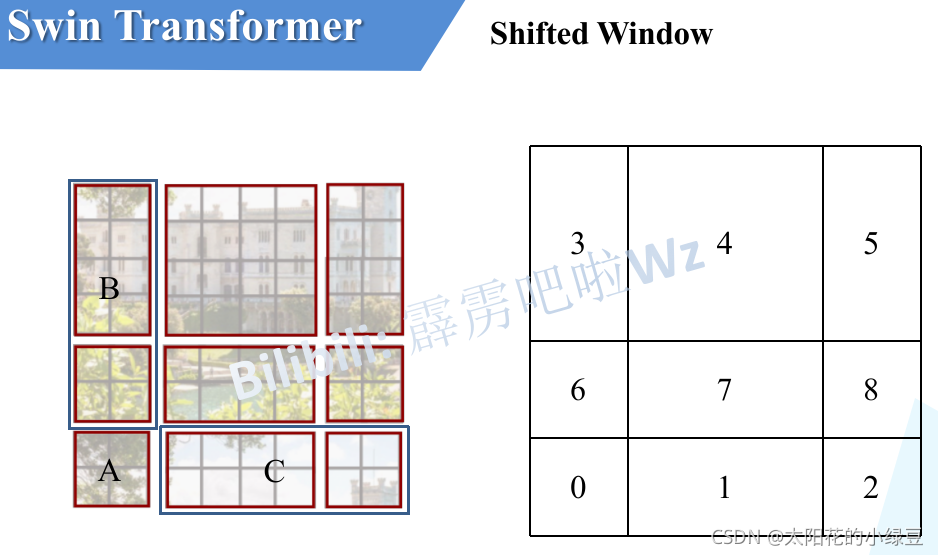
接着,再将区域A和B移至最右侧。

移动完后,4是一个单独的窗口;将5和3合并成一个窗口;7和1合并成一个窗口;8、6、2和0合并成一个窗口。这样又和原来一样是4个4x4的窗口了,所以能够保证计算量是一样的。这里肯定有人会想,把不同的区域合并在一起(比如5和3)进行MSA,这信息不就乱窜了吗?是的,为了防止这个问题,在实际计算中使用的是masked MSA即带蒙板mask的MSA,这样就能够通过设置蒙板来隔绝不同区域的信息了。关于mask如何使用,可以看下下面这幅图,下图是以上面的区域5和区域3为例。
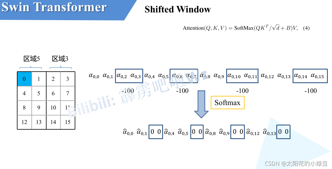
对于该窗口内的每一个像素(或称token,patch)在进行MSA计算时,都要先生成对应的query(q),key(k),value(v)。假设对于上图的像素0而言,得到 后要与每一个像素的k进行匹配(match),假设
代表
与像素0对应的
进行匹配的结果,那么同理可以得到
至
。按照普通的MSA计算,接下来就是SoftMax操作了。但对于这里的masked MSA,像素0是属于区域5的,我们只想让它和区域5内的像素进行匹配。那么我们可以将像素0与区域3中的所有像素匹配结果都减去100(例如
等等),由于α的值都很小,一般都是零点几的数,将其中一些数减去100后在通过SoftMax得到对应的权重都等于0了。所以对于像素0而言实际上还是只和区域5内的像素进行了MSA。那么对于其他像素也是同理,具体代码是怎么实现的,后面会在代码讲解中进行详解。注意,在计算完后还要把数据给挪回到原来的位置上(例如上述的A,B,C区域)。
5 Relative Position Bias详解
关于相对位置偏执,论文里也没有细讲,就说了参考的哪些论文,然后说使用了相对位置偏执后给够带来明显的提升。根据原论文中的表4可以看出,在Imagenet数据集上如果不使用任何位置偏执,top-1为80.1,但使用了相对位置偏执(rel. pos.)后top-1为83.3,提升还是很明显的。
那这个相对位置偏执是加在哪的呢,根据论文中提供的公式可知是在Q和K进行匹配并除以后加上了相对位置偏执B。
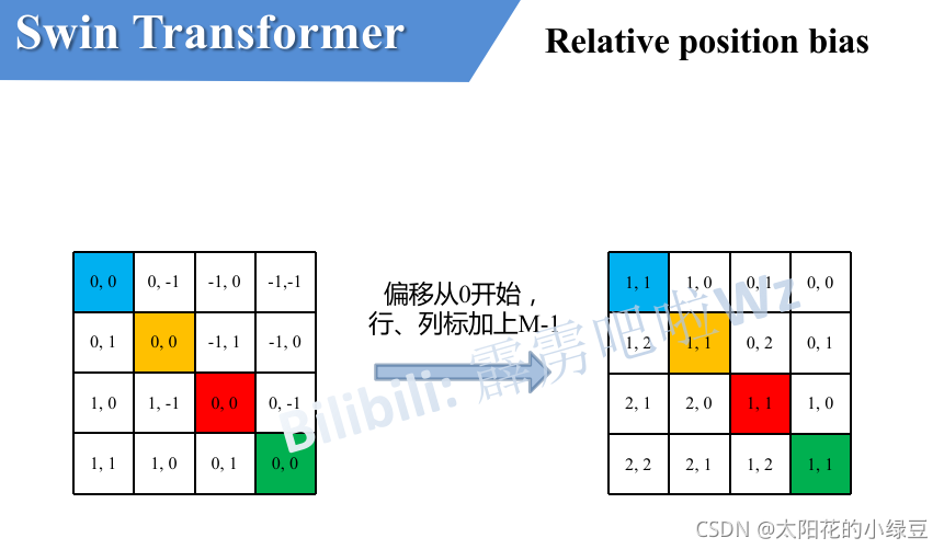
由于论文中并没有详解讲解这个相对位置偏执,所以我自己根据阅读源码做了简单的总结。如下图,假设输入的feature map高宽都为2,那么首先我们可以构建出每个像素的绝对位置(左下方的矩阵),对于每个像素的绝对位置是使用行号和列号表示的。比如蓝色的像素对应的是第0行第0列所以绝对位置索引是( 0 , 0 ) (0,0)(0,0),接下来再看看相对位置索引。首先看下蓝色的像素,在蓝色像素使用q与所有像素k进行匹配过程中,是以蓝色像素为参考点。然后用蓝色像素的绝对位置索引与其他位置索引进行相减,就得到其他位置相对蓝色像素的相对位置索引。例如黄色像素的绝对位置索引是( 0 , 1 ) (0,1)(0,1),则它相对蓝色像素的相对位置索引为( 0 , 0 ) − ( 0 , 1 ) = ( 0 , − 1 ) (0, 0) - (0, 1)=(0, -1)(0,0)−(0,1)=(0,−1),这里是严格按照源码中来讲的,请不要杠。那么同理可以得到其他位置相对蓝色像素的相对位置索引矩阵。同样,也能得到相对黄色,红色以及绿色像素的相对位置索引矩阵。接下来将每个相对位置索引矩阵按行展平,并拼接在一起可以得到下面的4x4矩阵 。

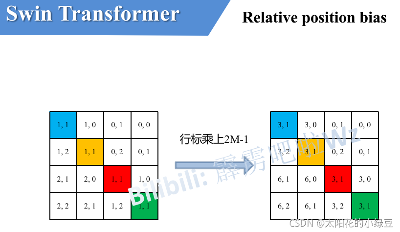
请注意,我这里描述的一直是相对位置索引,并不是相对位置偏执参数。因为后面我们会根据相对位置索引去取对应的参数。比如说黄色像素是在蓝色像素的右边,所以相对蓝色像素的相对位置索引为( 0 , − 1 ) (0, -1)(0,−1)。绿色像素是在红色像素的右边,所以相对红色像素的相对位置索引为( 0 , − 1 ) (0, -1)(0,−1)。可以发现这两者的相对位置索引都是( 0 , − 1 ) (0, -1)(0,−1),所以他们使用的相对位置偏执参数都是一样的。其实讲到这基本已经讲完了,但在源码中作者为了方便把二维索引给转成了一维索引。具体这么转的呢,有人肯定想到,简单啊直接把行、列索引相加不就变一维了吗?比如上面的相对位置索引中有( 0 , − 1 ) (0, -1)(0,−1)和( − 1 , 0 ) (-1,0)(−1,0)在二维的相对位置索引中明显是代表不同的位置,但如果简单相加都等于-1那不就出问题了吗?接下来我们看看源码中是怎么做的。首先在原始的相对位置索引上加上M-1(M为窗口的大小,在本示例中M=2),加上之后索引中就不会有负数了。
接着将所有的行标都乘上2M-1。
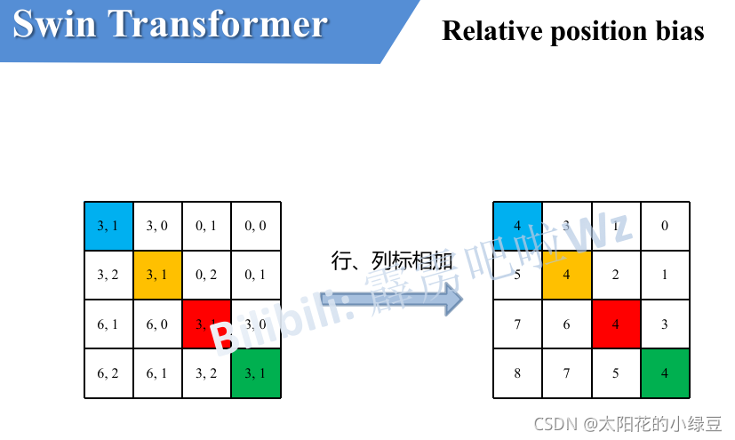
最后将行标和列标进行相加。这样即保证了相对位置关系,而且不会出现上述0 + ( − 1 ) = ( − 1 ) + 0 0+(-1)=(-1)+00+(−1)=(−1)+0的问题了,是不是很神奇。
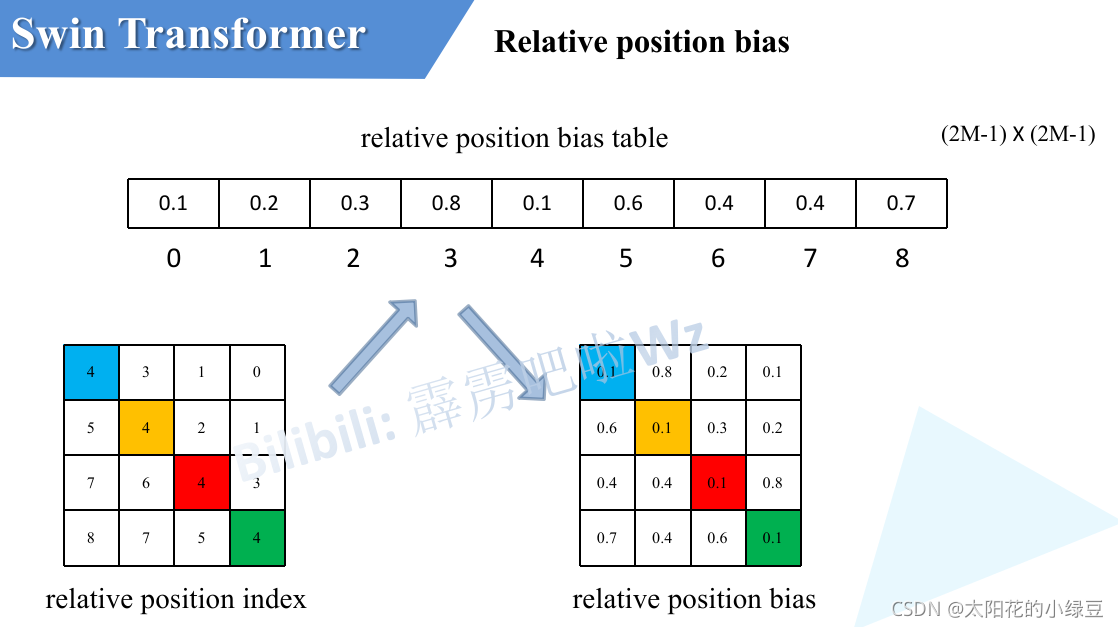
刚刚上面也说了,之前计算的是相对位置索引,并不是相对位置偏执参数。真正使用到的可训练参数是保存在relative position bias table表里的,这个表的长度是等于( 2 M − 1 ) × ( 2 M − 1 ) 的。那么上述公式中的相对位置偏执参数B是根据上面的相对位置索引表根据查relative position bias table表得到的,如下图所示。
6 模型详细配置参数
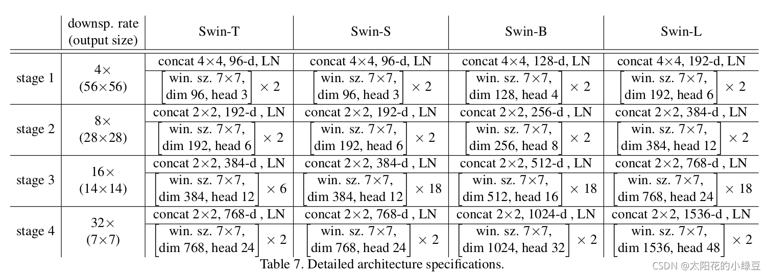
下图(表7)是原论文中给出的关于不同Swin Transformer的配置,T(Tiny),S(Small),B(Base),L(Large),其中:
- win. sz. 7x7表示使用的窗口(Windows)的大小
- dim表示feature map的channel深度(或者说token的向量长度)
- head表示多头注意力模块中head的个数
源码:
最后我们来看下 WindowAttention的实现。这里的实现只需要注意两点,就是pos编码设计和transform里面不同。
1. 设计了个相对位置编码bias表格
class WindowAttention(nn.Module):

    def __init__(self, dim, window_size, num_heads, qkv_bias=True, qk_scale=None, attn_drop=0., proj_drop=0.):

        super().__init__()
        self.dim = dim
        self.window_size = window_size  # Wh, Ww
        self.num_heads = num_heads
        head_dim = dim // num_heads
        self.scale = qk_scale or head_dim ** -0.5

        # define a parameter table of relative position bias
        # 设计了一个相对位置编码  相对位置编码个数 (2 * window_size - 1) * (2 * window_size - 1)
        # 因为在一个 7 * 7 的 window内  相对位置范围 (-6, 6) 有 2 * 7 - 1 = 13 个
        # 所以对于二维数据 应该有 13 * 13 个 即 (2w - 1) * (2w - 1) 也就是相对坐标范围应该为 0 ~ (2w - 1) * (2w - 1) - 1
        self.relative_position_bias_table = nn.Parameter(
            torch.zeros((2 * window_size[0] - 1) * (2 * window_size[1] - 1), num_heads))  # 2*Wh-1 * 2*Ww-1, nH

        # get pair-wise relative position index for each token inside the window
        # 得到 window 内的表格坐标
        coords_h = torch.arange(self.window_size[0])
        coords_w = torch.arange(self.window_size[1])
        coords = torch.stack(torch.meshgrid([coords_h, coords_w]))  # 2, Wh, Ww
        # 下面两行其实和 mask生成的是做的操作类似  也就是将数据展平后 广播后相减 得到相对坐标
        coords_flatten = torch.flatten(coords, 1)  # 2, Wh*Ww
        relative_coords = coords_flatten[:, :, None] - coords_flatten[:, None, :]  # 2, Wh*Ww, Wh*Ww
        relative_coords = relative_coords.permute(1, 2, 0).contiguous()  # Wh*Ww, Wh*Ww, 2
        # 但是上面的相对坐标和定义的 relative_position_bias_table还对应不上 relative_coords 取值范围 (-w + 1) ~ (w - 1)
        # 所以在dim=[1, 2] 维度 才加上 self.window_size[0] - 1 取值范围 变成 0 ~ (2w - 2)
        relative_coords[:, :, 0] += self.window_size[0] - 1  # shift to start from 0
        relative_coords[:, :, 1] += self.window_size[1] - 1
        # 最后在 dim=2 的维度上 乘以 2w - 1 所以在这个维度上取值范围为 0 ~  (2w - 2) * (2w - 1) = (2w - 1)**2 - (2w - 1)
        relative_coords[:, :, 0] *= 2 * self.window_size[1] - 1
        # 最后求和后得到的相对坐标范围 0 ~ (2w - 1)**2 - (2w - 1) + (2w - 2) = (2w - 1)**2 - 1
        # OKay 到此为止终于得到范围为 0 ~ (2w - 1)**2 - 1 和 上面的 relative_position_bias_table对应上了
        # 所以每次只需要用相对索引去 relative_position_bias_table 表格中取值就行了
        relative_position_index = relative_coords.sum(-1)  # Wh*Ww, Wh*Ww
        self.register_buffer("relative_position_index", relative_position_index)

        self.qkv = nn.Linear(dim, dim * 3, bias=qkv_bias)
        self.attn_drop = nn.Dropout(attn_drop)
        self.proj = nn.Linear(dim, dim)
        self.proj_drop = nn.Dropout(proj_drop)

        trunc_normal_(self.relative_position_bias_table, std=.02)
        self.softmax = nn.Softmax(dim=-1)
2. 添加位置编码信息的位置不同,这里是在 计算 qk.T后在加上位置编码 bias
attn = (q @ k.transpose(-2, -1))

relative_position_bias = self.relative_position_bias_table[self.relative_position_index.view(-1)].view(
    self.window_size[0] * self.window_size[1], self.window_size[0] * self.window_size[1], -1)  # Wh*Ww,Wh*Ww,nH
relative_position_bias = relative_position_bias.permute(2, 0, 1).contiguous()  # nH, Wh*Ww, Wh*Ww
attn = attn + relative_position_bias.unsqueeze(0)
其他的就和普通的 self attention 差不多 这里就不进行分析了。
到此为止源码基本分析完!
从代码上我们可以看到,Swin Transformer 基本上是抛弃了卷积操作。但一个SW-MSA确又看到了卷积的影子。
SwinTransformV2 已经推出,用于大模型。对网络结构也做了一些调整。

旨在为数千万中国开发者提供一个无缝且高效的云端环境,以支持学习、使用和贡献开源项目。
更多推荐


 0
0 0
0- 0


 已为社区贡献1条内容

所有评论(0)