因果推断笔记——因果图建模之微软开源的EconML(五)
微软EconML简介:基于机器学习的Heterogeneous Treatment Effects估计机器学习最大的promise之一是在许多领域实现决策的自动化。许多数据驱动的决策场景的核心问题是对heterogeneous treatment effects的估计,也即:对于具有特定特征集的样本,干预对输出结果的causal effect是什么?简言之,这个Python工具包旨在:测量某些干预
文章目录
1 EconML介绍
微软EconML简介:基于机器学习的Heterogeneous Treatment Effects估计
GITHUB : microsoft/EconML
econml DOC:user guide
1.1 EconML介绍
机器学习最大的promise之一是在许多领域实现决策的自动化。
许多数据驱动的决策场景的核心问题是对heterogeneous treatment effects的估计,也即:对于具有特定特征集的样本,干预对输出结果的causal effect是什么?
简言之,这个Python工具包旨在:
- 测量某些干预变量T对结果变量Y的causal effect
- 控制一组特征X和W,来衡量causal effect如何随X的变化而变化
这个Python工具包旨在测量某些干预变量T对结果变量Y的causal effect,控制一组特征X和W,来衡量causal effect如何随X的变化而变化。
这个包里实现的方法适用于观察的数据集(非实验或历史)。为了使估计结果具有因果解释,一些算法假设数据中没有未观察到的混杂因子(即同时对T和Y产生影响的因子均被包含在X,W中),而其他一些算法则假设可以使用工具变量Z(即观测变量Z对干预T有影响,但对结果变量Y没有直接影响)。
并且包中的大多数算法都可以提供置信区间和推断结果。
我们将概述最近将机器学习与因果推理结合起来的方法,以及机器学习给因果推理估计方法带来的重要统计性能。
相比DoWhy,EconML借助一些更复杂的机器学习算法来进行因果推断。在EconML中可以使用的因果推断方法有:
- 双机器学习(Double Machine Learning)。
- 双重鲁棒学习(Doubly Robust Learner)。
- 树型学习器(Forest Learners)。
- 元学习器(Meta Learners)。
- 深度工具变量法(Deep IV).
- 正交随机树(Orthogonal Random Forest)
- 加权双机器学习(Weighted Double Machine Learning)
我们还将概述置信区间构建(例如自举、小袋自举、去偏lasso)、可解释性(形状值、树解释器)和策略学习(双鲁棒策略学习)的方法。
EconML希望做到以下几点:
- 实现同时涉及计量经济学和机器学习的最新方法
- 保持对effect heterogeneity建模的灵活性(通过随机森林、boosting、lasso和神经网络等技术),同时- 保留所学模型的因果解释,并同时提供有效的置信区间
- 使用统一的API
- 构建标准的Python包以用于机器学习和数据分析
1.2 一些理论解答
参考:
因果推断笔记—— 相关理论:Rubin Potential、Pearl、倾向性得分、与机器学习异同(二)的【3.0.2 章节】
异质处理效应 (Heterogenous treatment effects,HTE)
简单理解就是按某些规律进行分组之后的ATE,也就是“条件平均处理效应”(Conditional Average Treatment Effect,CATE)
每个子组的平均处理效应被称为“条件平均处理效应”(Conditional Average Treatment Effect,CATE) ,也就是说,每个子组的平均处理效应被称为条件平均处理效应,以子组内的分类方式为条件。
1.3 常规CATE的估计器
在econML中,“条件平均处理效应”(Conditional Average Treatment Effect,CATE) 的四种估计方式:
- 双机器学习(Double Machine Learning)。
- 双重鲁棒学习(Doubly Robust Learner)。
- 元学习器(Meta Learners)。
- 正交随机树(Orthogonal Random Forest)
DML的几种方法包括:
- econml.dml.DML(*, model_y, model_t, model_final) # 基础双重ML的模型
- econml.dml.LinearDML(*[, model_y, model_t, …]) # 线性估计器
- econml.dml.SparseLinearDML(*[, model_y, …]) # 稀疏线性估计器
- econml.dml.CausalForestDML(*[, model_y, …]) # 因果树
- econml.dml.NonParamDML(*, model_y, model_t, …) # 非参数ML估计器, that can have arbitrary final ML models of the CATE.
双重鲁棒学习(Doubly Robust Learner)几种方法:
- econml.dr.DRLearner(*[, model_propensity, …])
- econml.dr.LinearDRLearner(*[, …])
- econml.dr.SparseLinearDRLearner(*[, …])
- econml.dr.ForestDRLearner(*[, …])
CATE estimator that uses doubly-robust correction techniques to account for covariate shift (selection bias) between the treatment arms.
元学习器(Meta Learners)四种方法:
- econml.metalearners.XLearner(*, models[, …])
- econml.metalearners.TLearner(*, models[, …])
- econml.metalearners.SLearner(*, overall_model)
- econml.metalearners.DomainAdaptationLearner(*, …) 元算法,使用领域适应技术来解释
正交随机树(Orthogonal Random Forest) 的两种方法:
- econml.orf.DMLOrthoForest(*[, n_trees, …])
- econml.orf.DROrthoForest(*[, n_trees, …])
1.4 IV工具变量 + CATE的估计器
Double Machine Learning (DML) IV的几种方法:
- econml.iv.dml.OrthoIV(*[, model_y_xw, …])
用IV实现正交/双ml方法进行CATE估计 - econml.iv.dml.DMLIV(*[, model_y_xw, …])
参数DMLIV估计器的基类来估计一个CATE。 - econml.iv.dml.NonParamDMLIV(*[, model_y_xw, …])
非参数DMLIV的基类,允许在DMLIV算法的最后阶段采用任意平方损耗的ML方法。
Doubly Robust (DR) IV 稳健+IV几种方法:
- econml.iv.dr.DRIV(*[, model_y_xw, …])
- econml.iv.dr.LinearDRIV(*[, model_y_xw, …])
- econml.iv.dr.SparseLinearDRIV(*[, …]) # 稀疏
- econml.iv.dr.ForestDRIV(*[, model_y_xw, …]) # 因果树
- econml.iv.dr.IntentToTreatDRIV(*[, …])
- econml.iv.dr.LinearIntentToTreatDRIV(*[, …]) # 为线性意图处理A/B测试设置实现DRIV算法
DeepIV方法:
- econml.iv.nnet.DeepIV(*, n_components, m, h, …)
Sieve Methods 的几种方法:
- econml.iv.sieve.SieveTSLS(*, t_featurizer, …)
- econml.iv.sieve.HermiteFeatures(degree[, …])
- econml.iv.sieve.DPolynomialFeatures([…])
1.5 动态处理效应的估计器
- econml.dynamic.dml.DynamicDML(*[, model_y, …])
用于动态处理效果估计的CATE估计器。
2 智能营销案例一:(econml)不同优惠折扣下的用户反应
参考:Case Study - Customer Segmentation at An Online Media Company.ipynb
2.1 背景

如今,商业决策者依靠评估干预的因果效应来回答有关策略转变的假设问题,比如打折促销特定产品、向网站添加新功能或增加销售团队的投资。
然而,人们越来越感兴趣的是了解不同用户对这两种选择的不同反应,而不是学习是否要针对所有用户的特定干预采取行动。 识别对干预反应最强烈的用户特征,有助于制定规则,将未来用户划分为不同的群体。 这可以帮助优化政策,使用最少的资源,获得最大的利润。
在本案例研究中,我们将使用一个个性化定价示例来解释EconML库如何适应这个问题,并提供健壮可靠的因果解决方案。
目的是了解不同收入水平人群的需求的异质性价格弹性,了解哪个用户对小折扣的反应最强烈。
此外,他们的最终目标是确保,尽管对一些消费者降低了价格,但需求有足够的提高,以提高整体收入。
EconML的基于“DML”的估计器可用于获取现有数据中的折扣变化,以及一组丰富的用户特性,以估计随多个客户特性而变化的异构价格敏感性。
然后,EconML的可解释性的两个函数:
- SingleTreeCateInterpreter
提供了一个presentation-ready总结的关键特性,解释折扣最大的响应能力的差异, - SingleTreePolicyInterpreter
- 建议谁应该获得折扣政策为了增加收入(不仅需求),这可能有助于该公司在未来为这些用户设定一个最优价格。
2.2 数据准备与理解
# Some imports to get us started
# Utilities
import os
import urllib.request
import numpy as np
import pandas as pd

# Generic ML imports
from sklearn.preprocessing import PolynomialFeatures
from sklearn.ensemble import GradientBoostingRegressor

# EconML imports
from econml.dml import LinearDML, CausalForestDML
from econml.cate_interpreter import SingleTreeCateInterpreter, SingleTreePolicyInterpreter

import matplotlib.pyplot as plt

%matplotlib inline

# Import the sample pricing data
file_url = "https://msalicedatapublic.blob.core.windows.net/datasets/Pricing/pricing_sample.csv"
train_data = pd.read_csv(file_url)

# Define estimator inputs
Y = train_data["demand"]  # outcome of interest
T = train_data["price"]  # intervention, or treatment
X = train_data[["income"]]  # features
W = train_data.drop(columns=["demand", "price", "income"])  # confounders
# Get test data
X_test = np.linspace(0, 5, 100).reshape(-1, 1)
X_test_data = pd.DataFrame(X_test, columns=["income"])
其中train_data是10000*11完整的数据集,而X_test_data是新生成的一列自变量X,
这里可以看到,test数据集 其实不用捎上混杂因子的W变量们,也不用额外生成干预变量T
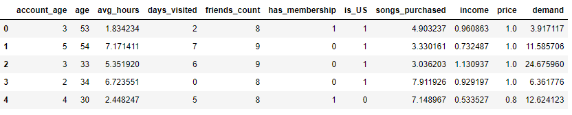
数据格式为:
| Feature Name | Type | Details |
|---|---|---|
| account_age | W | user’s account age |
| age | W | user’s age |
| avg_hours | W | the average hours user was online per week in the past |
| days_visited | W | the average number of days user visited the website per week in the past |
| friend_count | W | number of friends user connected in the account |
| has_membership | W | whether the user had membership |
| is_US | W | whether the user accesses the website from the US |
| songs_purchased | W | the average songs user purchased per week in the past |
| income | X | user’s income |
| price | T | the price user was exposed during the discount season (baseline price * small discount) |
| demand | Y | songs user purchased during the discount season |
数据集*有~ 10000个观察,包括9个连续和分类变量,代表用户的特征和在线行为历史,如年龄,日志收入,以前的购买,每周以前的在线时间等。
为了保护公司的隐私,我们这里以模拟数据为例。数据是综合生成的,特征分布与真实分布不一致。
然而,特征名称保留了它们的名称和含义.
这里来盘一下具体的因果逻辑:
- 其他变量:account_age ~ songs_purchased - W - 混杂因子
- income - X - 考察变量 - 用户收入
- demand - Y - outcome - 销量
- Price - T - 干预,折扣,取值为
[1,0.9,0.8],根据下面的公式的来
T = { 1 with p = 0.2 , 0.9 with p = 0.3 , if income < 1 0.8 with p = 0.5 , 1 with p = 0.7 , 0.9 with p = 0.2 , if income ≥ 1 0.8 with p = 0.1 , T = \begin{cases} 1 & \text{with } p=0.2, \\ 0.9 & \text{with }p=0.3, & \text{if income}<1 \\ 0.8 & \text{with }p=0.5, \\ \\ 1 & \text{with }p=0.7, \\ 0.9 & \text{with }p=0.2, & \text{if income}\ge1 \\ 0.8 & \text{with }p=0.1, \\ \end{cases} T=⎩⎪⎪⎪⎪⎪⎪⎪⎪⎪⎪⎨⎪⎪⎪⎪⎪⎪⎪⎪⎪⎪⎧10.90.810.90.8with p=0.2,with p=0.3,with p=0.5,with p=0.7,with p=0.2,with p=0.1,if income<1if income≥1
2.3 生成假的Groud Truth的估计效应
估计效应的对比,此时没有一个标准答案,所以这里就搞了一个手算版本,当作真实的估计量,来进行对比。
{
γ
(
X
)
=
−
3
−
14
⋅
{
income
<
1
}
β
(
X
,
W
)
=
20
+
0.5
⋅
avg-hours
+
5
⋅
{
day-svisited
>
4
}
\begin{cases} \gamma(X) = -3 - 14 \cdot \{\text{income}<1\} \\ \beta(X,W) = 20 + 0.5 \cdot \text{avg-hours} + 5 \cdot \{\text{day-svisited}>4\} \\ \end{cases}
{γ(X)=−3−14⋅{income<1}β(X,W)=20+0.5⋅avg-hours+5⋅{day-svisited>4}
最终要算的是价格弹性elasticity
Y
=
γ
(
X
)
⋅
T
+
β
(
X
,
W
)
e
l
a
s
t
i
c
i
t
y
(
手
算
)
=
(
γ
(
X
)
⋅
T
)
/
Y
Y = \gamma(X) \cdot T + \beta(X,W) \\ elasticity(手算) = (\gamma(X) \cdot T) / Y
Y=γ(X)⋅T+β(X,W)elasticity(手算)=(γ(X)⋅T)/Y
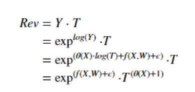
当然,在实际计算中有取对数的操作,公式会变成:
l
o
g
(
Y
)
=
θ
(
X
)
⋅
l
o
g
(
T
)
+
f
(
X
,
W
)
+
ϵ
l
o
g
(
T
)
=
g
(
X
,
W
)
+
η
log(Y) = \theta(X) \cdot log(T) + f(X,W) + \epsilon \\ log(T) = g(X,W) + \eta \\
log(Y)=θ(X)⋅log(T)+f(X,W)+ϵlog(T)=g(X,W)+η
整体生成手算的估计效应:
# Define underlying treatment effect function given DGP
def gamma_fn(X):
    return -3 - 14 * (X["income"] < 1)

def beta_fn(X):
    return 20 + 0.5 * (X["avg_hours"]) + 5 * (X["days_visited"] > 4)

def demand_fn(data, T):
    Y = gamma_fn(data) * T + beta_fn(data)
    return Y

def true_te(x, n, stats):
    if x < 1:
        subdata = train_data[train_data["income"] < 1].sample(n=n, replace=True)
    else:
        subdata = train_data[train_data["income"] >= 1].sample(n=n, replace=True)
    te_array = subdata["price"] * gamma_fn(subdata) / (subdata["demand"])
    if stats == "mean":
        return np.mean(te_array)
    elif stats == "median":
        return np.median(te_array)
    elif isinstance(stats, int):
        return np.percentile(te_array, stats)

# Get the estimate and range of true treatment effect
truth_te_estimate = np.apply_along_axis(true_te, 1, X_test, 1000, "mean")  # estimate
truth_te_upper = np.apply_along_axis(true_te, 1, X_test, 1000, 95)  # upper level
truth_te_lower = np.apply_along_axis(true_te, 1, X_test, 1000, 5)  # lower level
这里的truth_te_estimate就是最终估计数字了,公式即为:
e
l
a
s
t
i
c
i
t
y
(
手
算
)
=
(
γ
(
X
)
⋅
T
)
/
Y
elasticity(手算) = (\gamma(X) \cdot T) / Y
elasticity(手算)=(γ(X)⋅T)/Y
te_array = subdata["price"] * gamma_fn(subdata) / (subdata["demand"])
2.4 X~Y 分析:线性估计器LinearDML
# Get log_T and log_Y
log_T = np.log(T)
log_Y = np.log(Y)

# Train EconML model
est = LinearDML(
    model_y=GradientBoostingRegressor(),
    model_t=GradientBoostingRegressor(),
    featurizer=PolynomialFeatures(degree=2, include_bias=False),
)
est.fit(log_Y, log_T, X=X, W=W, inference="statsmodels")
# Get treatment effect and its confidence interval    得到治疗效果及其置信区间
te_pred = est.effect(X_test)
# 因为是配对实验,PSM,那就是 ps(y=1) - ps(y=0),每个人都有,
# 后面求ATE的时候,会进行平均
te_pred_interval = est.effect_interval(X_test)   # 置信区间 上限与下限


# Compare the estimate and the truth
plt.figure(figsize=(10, 6))
plt.plot(X_test.flatten(), te_pred, label="Sales Elasticity Prediction")
plt.plot(X_test.flatten(), truth_te_estimate, "--", label="True Elasticity")
plt.fill_between(
    X_test.flatten(),
    te_pred_interval[0],
    te_pred_interval[1],
    alpha=0.2,
    label="95% Confidence Interval",
)
plt.fill_between(
    X_test.flatten(),
    truth_te_lower,
    truth_te_upper,
    alpha=0.2,
    label="True Elasticity Range",
)
plt.xlabel("Income")
plt.ylabel("Songs Sales Elasticity")
plt.title("Songs Sales Elasticity vs Income")
plt.legend(loc="lower right")
先来解读一下步骤,LinearDML初始化之后,就直接fit建模,
这里初始化了model_y + model_t两个模型,也就是在估计器里,当出现了X/T/W/Y拟合了两个模型:
l
o
g
(
Y
)
=
θ
(
X
)
⋅
l
o
g
(
T
)
+
f
(
X
,
W
)
+
ϵ
l
o
g
(
T
)
=
g
(
X
,
W
)
+
η
log(Y) = \theta(X) \cdot log(T) + f(X,W) + \epsilon \\ log(T) = g(X,W) + \eta \\
log(Y)=θ(X)⋅log(T)+f(X,W)+ϵlog(T)=g(X,W)+η
此时可以说,X|T~Y的异质性处理效应就是弹性
(笔者喜欢在这里把X叫做异质变量,异质处理效应在这里就是需求弹性 ),
直接计算处理效应:est.effect(X_test),这里可以看到估计效应只需要X(income)一列就可以了,
同时给到处理效应的区间估计effect_interval,
之后就是把,手算的真效应估计量,pred预测估计量进行对比:

从手算的弹性~income的关系来看,是一条非线性曲线,当收入小于1时,弹性在-1.75左右,当收入大于1时,有一个较小的负值。
模型拟合的是二次项的函数,拟合不是很好。
但它仍然抓住了总体趋势:弹性是负的,如果人们有更高的收入,他们对价格变化的敏感度就会降低。
# Get the final coefficient and intercept summary
est.summary()
输出结果:

“线性dml”估计器也可以返回最终模型的系数和截距的总结,包括点估计、p值和置信区间。
由上表可知,
i
n
c
o
m
e
income
income具有正效应,
i
n
c
o
m
e
2
{income}^2
income2具有负效应,两者在统计学上都是显著的。
这里的两个结果,coef 和 CATE分别代表了 X -> Y 和 T -> Y的影响
CATE的代表有优惠券则会降低销量。
2.5 X~Y 分析:非线性估计器:因果树CausalForestDML
# Train EconML model
est = CausalForestDML(
    model_y=GradientBoostingRegressor(), model_t=GradientBoostingRegressor()
)
est.fit(log_Y, log_T, X=X, W=W, inference="blb")
# Get treatment effect and its confidence interval
te_pred = est.effect(X_test)
te_pred_interval = est.effect_interval(X_test)

# Compare the estimate and the truth
plt.figure(figsize=(10, 6))
plt.plot(X_test.flatten(), te_pred, label="Sales Elasticity Prediction")
plt.plot(X_test.flatten(), truth_te_estimate, "--", label="True Elasticity")
plt.fill_between(
    X_test.flatten(),
    te_pred_interval[0],
    te_pred_interval[1],
    alpha=0.2,
    label="95% Confidence Interval",
)
plt.fill_between(
    X_test.flatten(),
    truth_te_lower,
    truth_te_upper,
    alpha=0.2,
    label="True Elasticity Range",
)
plt.xlabel("Income")
plt.ylabel("Songs Sales Elasticity")
plt.title("Songs Sales Elasticity vs Income")
plt.legend(loc="lower right")

我们注意到,这个模型比“线性dml”更适合,95%置信区间正确地覆盖了真实的处理效果估计,并捕捉了收入约为1时的变化。
总体而言,该模型表明,低收入人群比高收入人群对价格变化更加敏感。
2.6 X|T~Y分析:SingleTreeCateInterpreter哪些用户比较积极/消极
EconML包括可解释性工具,以更好地理解治疗效果。
官方可解释性Interpretability的文章中提到:
:class:.SingleTreeCateInterpretertrains a single shallow decision tree for the treatment effect θ ( X ) \theta(X) θ(X) you learned from any of our available CATE estimators on a small set of feature X that you are interested to learn heterogeneity from.
The model will split on the cutoff points that maximize the treatment effect difference in each leaf.
Finally each leaf will be a subgroup of samples that respond to a treatment differently from other leaves.
治疗效果可能很复杂,但我们通常感兴趣的是一些简单的规则,这些规则可以区分哪些用户对提议的变化做出积极回应,哪些用户保持中立,哪些用户做出消极回应。
EconML SingleTreeCateInterpreter通过训练由任何EconML估计器输出的处理效果的单一决策树来提供可解释性。
intrp = SingleTreeCateInterpreter(include_model_uncertainty=True, max_depth=2, min_samples_leaf=10)
intrp.interpret(est, X_test)
plt.figure(figsize=(25, 5))
intrp.plot(feature_names=X.columns, fontsize=12)
在下图中,我们可以看到暗红色的用户(income < 0.48)对折扣反应强烈,白色的用户对折扣反应轻微。

SingleTreeCateInterpreter 与 SingleTreePolicyInterpreter 的差异:
- 前者代表,根据处理效应,拆分人群,人群之间的差距较大;
- 后者代表,找出 能发券 / 不能发券的界限
2.7 T~X分析:SingleTreePolicyInterpreter 什么收入的人该打折
该模型的解释,参考Interpretability,找出 该发 or 不该发优惠券的群体:
Instead of fitting a tree to learn groups that have a different treatment effect(上个模块SingleTreeCateInterpreter的含义), :class:.SingleTreePolicyInterpretertries to split the samples into different treatment groups.
So in the case of binary treatments it tries to create sub-groups such that all samples within the group have either all positive effect or all negative effect.
Thus it tries to separate responders from non-responders, as opposed to trying to find groups that have different levels of response.
This way you can construct an interpretable personalized policy where you treat the groups with a postive effect and don’t treat the group with a negative effect. Our policy tree provides the recommended treatment at each leaf node.
我们希望做出政策决定,使收入最大化,而不是需求最大化。
在这个场景中,收入的计算公式为:
随着价格的降低,只有当
θ
(
X
)
+
1
<
0
\theta(X)+1<0
θ(X)+1<0时,收入才会增加。
因此,我们在这里设置sample_treatment_cast=-1,以了解我们应该给哪种类型的客户一个小的折扣,以使收入最大。
sample_treatment_cast对其进行解释,econml文档原表达:
sample_treatment_costs is the cost of treatment. Policy will treat if effect is above this cost.
intrp = SingleTreePolicyInterpreter(risk_level=0.05, max_depth=2, min_samples_leaf=1, min_impurity_decrease=0.001)
intrp.interpret(est, X_test, sample_treatment_costs=-1)
plt.figure(figsize=(25, 5))
intrp.plot(feature_names=X.columns, treatment_names=["Discount", "No-Discount"], fontsize=12)
EconML库包括“SingleTreePolicyInterpreter”等策略可解释性工具,该工具可以计算治疗成本和治疗效果,以了解关于哪些客户可以获利的简单规则。
从下图中我们可以看到,模型建议对收入低于
0.985
0.985
0.985的人给予折扣,对其他人给予原价。

SingleTreeCateInterpreter 与 SingleTreePolicyInterpreter 的差异:
- 前者代表,根据处理效应,拆分人群,人群之间的差距较大;
- 后者代表,找出 能发券 / 不能发券的界限
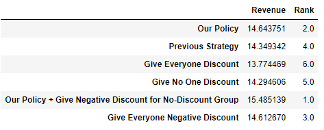
2.8 干预后的结果对比(该打折的人打折后)
现在,让我们将我们的政策与其他基准政策进行比较,
我们的模型告诉我们哪些用户可以给予小的折扣,在这个实验中,我们会为这些用户设定10%的折扣级别。
由于模型被错误地指定,我们不会期望有大折扣的好结果。
在这里,因为我们知道基本的真相,所以我们可以评估这个政策的价值。
# define function to compute revenue
def revenue_fn(data, discount_level1, discount_level2, baseline_T, policy):
    policy_price = baseline_T * (1 - discount_level1) * policy + baseline_T * (1 - discount_level2) * (1 - policy)
    demand = demand_fn(data, policy_price)
    rev = demand * policy_price
    return rev

policy_dic = {}
# our policy above
policy = intrp.treat(X)
policy_dic["Our Policy"] = np.mean(revenue_fn(train_data, 0, 0.1, 1, policy))

## previous strategy
policy_dic["Previous Strategy"] = np.mean(train_data["price"] * train_data["demand"])

## give everyone discount
policy_dic["Give Everyone Discount"] = np.mean(revenue_fn(train_data, 0.1, 0, 1, np.ones(len(X))))

## don't give discount
policy_dic["Give No One Discount"] = np.mean(revenue_fn(train_data, 0, 0.1, 1, np.ones(len(X))))

## follow our policy, but give -10% discount for the group doesn't recommend to give discount
policy_dic["Our Policy + Give Negative Discount for No-Discount Group"] = np.mean(revenue_fn(train_data, -0.1, 0.1, 1, policy))

## give everyone -10% discount
policy_dic["Give Everyone Negative Discount"] = np.mean(revenue_fn(train_data, -0.1, 0, 1, np.ones(len(X))))

# get policy summary table
res = pd.DataFrame.from_dict(policy_dic, orient="index", columns=["Revenue"])
res["Rank"] = res["Revenue"].rank(ascending=False)
res
这里面的一顿操作有点费解的是,intrp.treat(X)这个输出的是什么:
每个人是否要进行打折,根据SingleTreePolicyInterpreter来判定,输出内容[0,1],这里的每个人指的是训练集的X,至于打多少折,这里默认为0.1
里面还有一组很骚气的组,Our Policy + Give Negative Discount for No-Discount Group,竟然敢对不推荐给折扣的人涨价,当然revenue是上去的,rank排名第1。
输出结果:
3 智能营销案例二:(econml+dowhy)不同优惠折扣下的用户反应
是上面的案例【智能营销案例一:(econml)不同优惠折扣下的用户反应】的延申,一些数据计算过程都与上面一致,所以一些内容我就不赘述了。
链接:Case Study - Customer Segmentation at An Online Media Company - EconML + DoWhy.ipynb
类似的dowhy + econml的案例也可以看:
3.1 背景
如【2.1】
3.2 数据准备与理解
如【2.2】
3.3 生成假的Groud Truth的估计效应
如【2.3】
3.4 利用dowhy创建因果图 + EconML创建线性估计器LinearDML
这里因为econml和dowhy集成非常好,所以可以非常好的无缝衔接与使用。
那么dowhy主要是需要发挥其因果图方面的能力。
通过定义这些假设,DoWhy可以为我们生成一个因果图,并使用该图首先识别因果效应。
# initiate an EconML cate estimator
est = LinearDML(model_y=GradientBoostingRegressor(), model_t=GradientBoostingRegressor(),
              featurizer=PolynomialFeatures(degree=2, include_bias=False))

# fit through dowhy
est_dw = est.dowhy.fit(Y, T, X=X, W=W, outcome_names=["log_demand"], treatment_names=["log_price"], feature_names=["income"],
               confounder_names=confounder_names, inference="statsmodels")

# Visualize causal graph
try:
    # Try pretty printing the graph. Requires pydot and pygraphviz
    display(
        Image(to_pydot(est_dw._graph._graph).create_png())
    )
except:
    # Fall back on default graph view
    est_dw.view_model()
LinearDML是常规的econml的线性估计器,这里利用直接在估计器上再模拟一个因果图(est.dowhy.fit)
因果图这里就需要把,X/W/T都定义好,具体如下图:
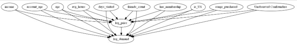
构建了因果图,就可以探索变量之间,有没有更深层的关系(前门、后门、IV):
identified_estimand = est_dw.identified_estimand_
print(identified_estimand)
输出如下:
Estimand type: nonparametric-ate

### Estimand : 1
Estimand name: backdoor1 (Default)
Estimand expression:
     d
────────────(Expectation(log_demand|is_US,has_membership,days_visited,age,inco
d[log_price]


me,account_age,avg_hours,songs_purchased,friends_count))

Estimand assumption 1, Unconfoundedness: If U→{log_price} and U→log_demand then P(log_demand|log_price,is_US,has_membership,days_visited,age,income,account_age,avg_hours,songs_purchased,friends_count,U) = P(log_demand|log_price,is_US,has_membership,days_visited,age,income,account_age,avg_hours,songs_purchased,friends_count)

### Estimand : 2
Estimand name: iv
No such variable found!
### Estimand : 3
Estimand name: frontdoor
No such variable found!
因为有定义混杂因子W,所以这里X -> Y,一般都是有后门路径的。
没有前门路径做阻断。
了解完变量之间的因果关系之后可以拿到具体的处理效应:
lineardml_estimate = est_dw.estimate_
print(lineardml_estimate)
输出为:
*** Causal Estimate ***

## Identified estimand
Estimand type: nonparametric-ate

### Estimand : 1
Estimand name: backdoor
Estimand expression:
     d
────────────(Expectation(log_demand|songs_purchased,avg_hours,days_visited,has
d[log_price]


_membership,account_age,age,income,is_US,friends_count))

Estimand assumption 1, Unconfoundedness: If U→{log_price} and U→log_demand then P(log_demand|log_price,songs_purchased,avg_hours,days_visited,has_membership,account_age,age,income,is_US,friends_count,U) = P(log_demand|log_price,songs_purchased,avg_hours,days_visited,has_membership,account_age,age,income,is_US,friends_count)

## Realized estimand
b: log_demand~log_price+songs_purchased+avg_hours+days_visited+has_membership+account_age+age+income+is_US+friends_count | income
Target units: ate

## Estimate
Mean value: -0.997133982212133
Effect estimates: [-1.09399505 -1.48371714 -0.83401226 ... -1.3358834  -1.91959094
 -0.40863328]
可以看到这里的CHTE的效应值为:-0.997133982212133
这里的效应是什么意思?
这里的效应是T -> Y,T = 1 / T = 0 的情况下,demand=Y的变量
以及与后面估计值有啥差异?
后面的是Y~(X|T)的变化,这里也就是弹性了
估计弹性,这个部分与【2.4】线性估计内容一致
# Get treatment effect and its confidence interval
te_pred = est_dw.effect(X_test).flatten()
te_pred_interval = est_dw.effect_interval(X_test)

# Compare the estimate and the truth
plt.figure(figsize=(10, 6))
plt.plot(X_test.flatten(), te_pred, label="Sales Elasticity Prediction")
plt.plot(X_test.flatten(), truth_te_estimate, "--", label="True Elasticity")
plt.fill_between(
    X_test.flatten(),
    te_pred_interval[0].flatten(),
    te_pred_interval[1].flatten(),
    alpha=0.2,
    label="95% Confidence Interval",
)
plt.fill_between(
    X_test.flatten(),
    truth_te_lower,
    truth_te_upper,
    alpha=0.2,
    label="True Elasticity Range",
)
plt.xlabel("Income")
plt.ylabel("Songs Sales Elasticity")
plt.title("Songs Sales Elasticity vs Income")
plt.legend(loc="lower right")

3.5 EconML因果树估计器CausalForestDML + dowhy构建因果图
大部分与【2.5】一致,就是构造因果树估计器的同时,再额外构建因果图:
# initiate an EconML cate estimator
est_nonparam = CausalForestDML(model_y=GradientBoostingRegressor(), model_t=GradientBoostingRegressor())
# fit through dowhy
est_nonparam_dw = est_nonparam.dowhy.fit(Y, T, X=X, W=W, outcome_names=["log_demand"], treatment_names=["log_price"],
                                         feature_names=["income"], confounder_names=confounder_names, inference="blb")
3.6 dowhy基于因果树的估计稳定性检验:反驳
具体可参考:因果推断笔记——因果图建模之微软开源的dowhy(一)
大致的一些反驳的方式:
- 「添加随机混杂因子」:添加一个随机变量作为混杂因子后估计因果效应是否会改变(期望结果:不会)
- 「安慰剂干预」:将真实干预变量替换为独立随机变量后因果效应是否会改变(期望结果:因果效应归零)
- 「虚拟结果」:将真实结果变量替换为独立随机变量后因果效应是否会改变(期望结果:因果效应归零)
- 「模拟结果」:将数据集替换为基于接近给定数据集数据生成过程的方式模拟生成的数据集后因果效应是否会改变(期望结果:与数据生成过程的效应参数相匹配)
- 「添加未观测混杂因子」:添加一个额外的与干预和结果相关的混杂因子后因果效应的敏感性(期望结果:不过度敏感)
- 「数据子集验证」:将给定数据集替换为一个随机子集后因果效应是否会改变(期望结果:不会)
- 「自助验证」:将给定数据集替换为同一数据集的自助样本后因果效应是否会改变(期望结果:不会)
# Add Random Common Cause
res_random = est_nonparam_dw.refute_estimate(method_name="random_common_cause")
print(res_random)

# Add Unobserved Common Cause
res_unobserved = est_nonparam_dw.refute_estimate(
    method_name="add_unobserved_common_cause",
    confounders_effect_on_treatment="linear",
    confounders_effect_on_outcome="linear",
    effect_strength_on_treatment=0.1,
    effect_strength_on_outcome=0.1,
)
print(res_unobserved)

#Replace Treatment with a Random (Placebo) Variable
res_placebo = est_nonparam_dw.refute_estimate(
    method_name="placebo_treatment_refuter", placebo_type="permute",
    num_simulations=3
)
print(res_placebo)
# Remove a Random Subset of the Data
res_subset = est_nonparam_dw.refute_estimate(
    method_name="data_subset_refuter", subset_fraction=0.8,
    num_simulations=3)
print(res_subset)
3.7 T~X分析:SingleTreePolicyInterpreter 什么收入的人该打折
【如2.7】
3.8 干预后的结果对比(该打折的人打折后)
【如2.8】
4 案例:EconML + SHAP丰富可解释性
类似于如何用SHAP解释黑箱预测机器学习模型,我们也可以解释黑箱效应异质性模型。这种方法解释了为什么异质因果效应模型对特定人群产生了较大或较小的效应值。是哪些特征导致了这种差异?
当模型被简洁地描述时,这个问题很容易解决,例如线性异质性模型的情况,人们可以简单地研究模型的系数。然而,当人们开始使用更具表现力的模型(如随机森林和因果森林)来建模效果异质性时,就会变得困难。SHAP值对于理解模型从训练数据中提取的影响异质性的主导因素有很大的帮助。
我们的软件包提供了与SHAP库的无缝集成。每个CateEstimator都有一个方法shap_values,它返回每个处理和结果对的估计器输出的SHAP值解释。
然后,可以使用SHAP库提供的大量可视化功能对这些值进行可视化。此外,只要有可能,我们的库就会为每种最终模型类型从SHAP库中调用快速专用算法,这可以大大减少计算时间。
4.1 单干预 - 单输出
## Ignore warnings
from econml.dml import CausalForestDML, LinearDML, NonParamDML
from econml.dr import DRLearner
from econml.metalearners import DomainAdaptationLearner, XLearner
from econml.iv.dr import LinearIntentToTreatDRIV
import numpy as np
import scipy.special
import matplotlib.pyplot as plt
import shap
from sklearn.ensemble import RandomForestRegressor, RandomForestClassifier
from sklearn.linear_model import Lasso

np.random.seed(123)
n_samples = 5000
n_features = 10
true_te = lambda X: (X[:, 0]>0) * X[:, 0]
X = np.random.normal(0, 1, size=(n_samples, n_features))
W = np.random.normal(0, 1, size=(n_samples, n_features))
T = np.random.binomial(1, scipy.special.expit(X[:, 0]))
y = true_te(X) * T + 5.0 * X[:, 0] + np.random.normal(0, .1, size=(n_samples,))
X_test = X[:min(100, n_samples)].copy()
X_test[:, 0] = np.linspace(np.percentile(X[:, 0], 1), np.percentile(X[:, 0], 99), min(100, n_samples))


# 因果树估计器
est = CausalForestDML(random_state=123)
est.fit(y, T, X=X, W=W)

# 线性估计器
est = LinearDML(random_state=123)
est.fit(y, T, X=X, W=W)

# 非参数
est = NonParamDML(model_y=RandomForestRegressor(min_samples_leaf=20, random_state=123),
                  model_t=RandomForestRegressor(min_samples_leaf=20, random_state=123),
                  model_final=RandomForestRegressor(min_samples_leaf=20, random_state=123),
                  random_state=123)
est.fit(y.ravel(), T.ravel(), X=X, W=W)

# 双重鲁棒学习
est = DRLearner(model_regression=RandomForestRegressor(min_samples_leaf=20, random_state=123),
                model_propensity=RandomForestClassifier(min_samples_leaf=20, random_state=123),
                model_final=RandomForestRegressor(min_samples_leaf=20, random_state=123),
                random_state=123)
est.fit(y.ravel(), T.ravel(), X=X, W=W)

# 元学习 DomainAdaptationLearner
est = DomainAdaptationLearner(models=RandomForestRegressor(min_samples_leaf=20, random_state=123),
                              final_models=RandomForestRegressor(min_samples_leaf=20, random_state=123),
                              propensity_model=RandomForestClassifier(min_samples_leaf=20, random_state=123))
est.fit(y.ravel(), T.ravel(), X=X)

# Xlearner 元学习
# Xlearner.shap_values uses a slow shap exact explainer, as there is no well defined final model
# for the XLearner method.
est = XLearner(models=RandomForestRegressor(min_samples_leaf=20, random_state=123),
               cate_models=RandomForestRegressor(min_samples_leaf=20, random_state=123),
               propensity_model=RandomForestClassifier(min_samples_leaf=20, random_state=123))
est.fit(y.ravel(), T.ravel(), X=X)

# 工具变量
est = LinearIntentToTreatDRIV(model_y_xw=RandomForestRegressor(min_samples_leaf=20, random_state=123),
                              model_t_xwz=RandomForestClassifier(min_samples_leaf=20, random_state=123),
                              flexible_model_effect=RandomForestRegressor(min_samples_leaf=20, random_state=123),
                              random_state=123)
est.fit(y.ravel(), T.ravel(), Z=T.ravel(), X=X, W=W)
输出一个图来看:
est = CausalForestDML(random_state=123)
est.fit(y, T, X=X, W=W)
shap_values = est.shap_values(X[:20])
shap.plots.beeswarm(shap_values['Y0']['T0'])
详细的SHAP可参考:机器学习模型可解释性进行到底 —— SHAP值理论(一)
特征密度散点图:beeswarm

下图中每一行代表一个特征,横坐标为Shap值。特征的排序是按照shap 的平均绝对值,对模型来说的最重要特征。宽的地方表示有大量的样本聚集。
一个点代表一个样本,颜色越红说明特征本身数值越大,颜色越蓝说明特征本身数值越小。
可以看做一种特征重要性的排列图,从这里可以看到X0重要性高(排位);
同时,X0值越大,对模型的效果影响越好(SHAP值为正)
4.2 多干预 - 多输出
# 数据生成
np.random.seed(123)
n_samples = 5000
n_features = 10
n_treatments = 2
n_outputs = 3
true_te = lambda X: np.hstack([(X[:, [0]]>0) * X[:, [0]],
                               np.ones((X.shape[0], n_treatments - 1))*np.arange(1, n_treatments).reshape(1, -1)])
X = np.random.normal(0, 1, size=(n_samples, n_features))
W = np.random.normal(0, 1, size=(n_samples, n_features))
T = np.random.normal(0, 1, size=(n_samples, n_treatments))
for t in range(n_treatments):
    T[:, t] = np.random.binomial(1, scipy.special.expit(X[:, 0]))
y = np.sum(true_te(X) * T, axis=1, keepdims=True) + 5.0 * X[:, [0]] + np.random.normal(0, .1, size=(n_samples, 1))
y = np.tile(y, (1, n_outputs))
for j in range(n_outputs):
    y[:, j] = (j + 1) * y[:, j]
X_test = X[:min(100, n_samples)].copy()
X_test[:, 0] = np.linspace(np.percentile(X[:, 0], 1), np.percentile(X[:, 0], 99), min(100, n_samples))

#
est = CausalForestDML(n_estimators=400, random_state=123)
est.fit(y, T, X=X, W=W)

#
shap_values = est.shap_values(X[:200])

#
plt.figure(figsize=(25, 15))
for j in range(n_treatments):
    for i in range(n_outputs):
        plt.subplot(n_treatments, n_outputs, i + j * n_outputs + 1)
        plt.title("Y{}, T{}".format(i, j))
        shap.plots.beeswarm(shap_values['Y' + str(i)]['T' + str(j)], plot_size=None, show=False)
plt.tight_layout()
plt.show()
这里可以看到有生成了三个outcome,两个干预T,直接使用CausalForestDML因果树估计器,
所以就有6种情况可以得到:

5 回顾-Econml官方折扣营销案例
同:
因果推断与反事实预测——利用DML进行价格弹性计算(二十四)
这里回顾一下econml的一个官方案例,因果推断笔记——因果图建模之微软开源的EconML(五) 之前记录过,
github链接为:Case Study - Customer Segmentation at An Online Media Company.ipynb
比较相关的另一篇:
因果推断笔记——DML :Double Machine Learning案例学习(十六)
当然本节不摘录,只是回顾一下该案例中的一些关于弹性系数的重要细节。
5.1 数据结构
数据格式为:
| Feature Name | Type | Details |
|---|---|---|
| account_age | W | user’s account age |
| age | W | user’s age |
| avg_hours | W | the average hours user was online per week in the past |
| days_visited | W | the average number of days user visited the website per week in the past |
| friend_count | W | number of friends user connected in the account |
| has_membership | W | whether the user had membership |
| is_US | W | whether the user accesses the website from the US |
| songs_purchased | W | the average songs user purchased per week in the past |
| income | X | user’s income |
| price | T | the price user was exposed during the discount season (baseline price * small discount) |
| demand | Y | songs user purchased during the discount season |
数据集*有~ 10000个观察,包括9个连续和分类变量,代表用户的特征和在线行为历史,如年龄,日志收入,以前的购买,每周以前的在线时间等。
那么这里的:
- 其他变量:Z/W - account_age ~ songs_purchased - W - 混杂因子
- income - X - 考察变量 - 用户收入
- demand - Y - outcome - 销量
- Price - T - 干预,折扣,取值为
[1,0.9,0.8],根据下面的公式的来
5.2 训练后的系数含义-> 收入弹性
# Get log_T and log_Y
log_T = np.log(T)
log_Y = np.log(Y)

# Train EconML model
est = LinearDML(
    model_y=GradientBoostingRegressor(),
    model_t=GradientBoostingRegressor(),
    featurizer=PolynomialFeatures(degree=2, include_bias=False),
)
est.fit(log_Y, log_T, X=X, W=W, inference="statsmodels")
# Get treatment effect and its confidence interval    得到治疗效果及其置信区间
te_pred = est.effect(X_test)

# Get the final coefficient and intercept summary
est.summary()
输出结果:
解读一下含义:
- 第一点,非常重要的是,Y和T都取了对数,这样是标准的弹性log-log公式,可以求得弹性系数
- 系数项是
income-X -> sale-Y即为需求-收入的弹性系数;- 当收入小于1时,弹性在-1.75左右
- 当收入大于1时,有一个较小的负值
- 观察P值,影响是显著的
- 截距项=CATE,此时为-3.02,则代表, Y ( T = 1 ) − Y ( T = 0 ) Y(T=1)-Y(T=0) Y(T=1)−Y(T=0)为负数,代表整体来看,有折扣反而对销量不利
另外,
这里可以看到,如果要考虑计算CATE,那么此时,最终所求的回归系数:
就是
销
量
Y
−
收
入
i
n
c
o
m
e
销量Y-收入income
销量Y−收入income的弹性系数,
而并非
销
量
Y
−
P
r
i
c
e
折
扣
销量Y-Price折扣
销量Y−Price折扣的价格弹性系数。
对比案例2,其中Q销量(Y),P价格(T),最终模型求得的就是价格弹性,此时为啥不能求价格弹性,而是收入~销量的弹性?
此时就要来看看,DML求ATE和CATE之间的差异了:
求ATE:
- 两个平行模型:M1(Y~X) 和 M2(T~X)
- Y i ~ = α + β 1 T i ~ + ϵ i \tilde{Y_i} = \alpha + \beta_1 \tilde{T_i} + \epsilon_i Yi~=α+β1Ti~+ϵi
求CATE:
- 仍然两个平行模型M1(Y~X) 和 M2(T~X)
- Y i ~ = α + β 1 T i ~ + β 2 X i T i ~ + ϵ i \tilde{Y_i} = \alpha + \beta_1 \tilde{T_i} + \pmb{\beta}_2 \pmb{X_i} \tilde{T_i} + \epsilon_i Yi~=α+β1Ti~+βββ2XiXiXiTi~+ϵi
从CATE的公式可以看到,线性回归在ATE求解的时候,只有T,那么在CATE求解的时候,是X|T的交互项,所以不是单纯的价格弹性
5.3 Uplift的CATE预测功能
额外参考Uplift相关文章:
智能营销增益(Uplift Modeling)模型——模型介绍(一)
主要是看:est.effect(X)
est.effect(np.array([[1],[1]]))
>>> array([6.07165998, 6.07165998])
其中我们来看一下est.effect(np.array([[1],[2]]),T0=0, T1=1) 算的是啥,
之前笔者也有点混淆,该函数算出的是CATE(或者我这边用异质性个体平均处理效应),在X=1下,Y(T=1)-Y(T=0) => CATE
而这个结果并不是跟之前机器学习里面的,model.predict(X)一样,而是一种增量的表现。所以,常用于价格弹性的计算。
那么笔者在本小节使用的是Uplift,要说明的是,Uplift模型中也是需要预测某些新样本的增量关系,
那么此时介绍的这个函数以及应用也是比较适配的
当然,比如此时,X=1下的CATE为:6.07
有着两种问题:
- 大于0,说明,X=1的情况下,有优惠券还是好的
- 那6.07这样的差异,属于明显差异还是不明显?该如何选择样本,这个econml后面有两个模块是来解释的这个的
5.4 SingleTreePolicyInterpreter 和SingleTreeCateInterpreter
贴一下两个模块的图:
5.4.1 X|T~Y分析:SingleTreeCateInterpreter哪些用户比较积极/消极
EconML包括可解释性工具,以更好地理解治疗效果。
官方可解释性Interpretability的文章中提到:
:class:.SingleTreeCateInterpretertrains a single shallow decision tree for the treatment effect θ ( X ) \theta(X) θ(X) you learned from any of our available CATE estimators on a small set of feature X that you are interested to learn heterogeneity from.
The model will split on the cutoff points that maximize the treatment effect difference in each leaf.
Finally each leaf will be a subgroup of samples that respond to a treatment differently from other leaves.
治疗效果可能很复杂,但我们通常感兴趣的是一些简单的规则,这些规则可以区分哪些用户对提议的变化做出积极回应,哪些用户保持中立,哪些用户做出消极回应。
EconML SingleTreeCateInterpreter通过训练由任何EconML估计器输出的处理效果的单一决策树来提供可解释性。
intrp = SingleTreeCateInterpreter(include_model_uncertainty=True, max_depth=2, min_samples_leaf=10)
intrp.interpret(est, X_test)
plt.figure(figsize=(25, 5))
intrp.plot(feature_names=X.columns, fontsize=12)
在下图中,我们可以看到暗红色的用户(income < 0.48)对折扣反应强烈,白色的用户对折扣反应轻微。
SingleTreeCateInterpreter 与 SingleTreePolicyInterpreter 的差异:
- 前者代表,根据处理效应,拆分人群,人群之间的差距较大;
- 后者代表,找出 能发券 / 不能发券的界限
5.4.2 T~X分析:SingleTreePolicyInterpreter 什么收入的人该打折
该模型的解释,参考Interpretability,找出 该发 or 不该发优惠券的群体:
Instead of fitting a tree to learn groups that have a different treatment effect(上个模块SingleTreeCateInterpreter的含义), :class:.SingleTreePolicyInterpretertries to split the samples into different treatment groups.
So in the case of binary treatments it tries to create sub-groups such that all samples within the group have either all positive effect or all negative effect.
Thus it tries to separate responders from non-responders, as opposed to trying to find groups that have different levels of response.
This way you can construct an interpretable personalized policy where you treat the groups with a postive effect and don’t treat the group with a negative effect. Our policy tree provides the recommended treatment at each leaf node.
我们希望做出政策决定,使收入最大化,而不是需求最大化。
在这个场景中,收入的计算公式为:
随着价格的降低,只有当
θ
(
X
)
+
1
<
0
\theta(X)+1<0
θ(X)+1<0时,收入才会增加。
因此,我们在这里设置sample_treatment_cast=-1,以了解我们应该给哪种类型的客户一个小的折扣,以使收入最大。
intrp = SingleTreePolicyInterpreter(risk_level=0.05, max_depth=2, min_samples_leaf=1, min_impurity_decrease=0.001)
intrp.interpret(est, X_test, sample_treatment_costs=-1)
plt.figure(figsize=(25, 5))
intrp.plot(feature_names=X.columns, treatment_names=["Discount", "No-Discount"], fontsize=12)
EconML库包括“SingleTreePolicyInterpreter”等策略可解释性工具,该工具可以计算治疗成本和治疗效果,以了解关于哪些客户可以获利的简单规则。
从下图中我们可以看到,模型建议对收入低于
0.985
0.985
0.985的人给予折扣,对其他人给予原价。
SingleTreeCateInterpreter 与 SingleTreePolicyInterpreter 的差异:
- 前者代表,根据处理效应,拆分人群,人群之间的差距较大;
- 后者代表,找出 能发券 / 不能发券的界限
5.4.3 小结
如果按照uplift使用场景,来看一下下图,营销敏感人群如何定义,是本节想要表达的:
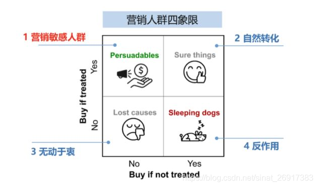
这里YY一下使用场景,假设我已经Train了一个优惠券/折扣 模型,然后对一批新样本计算uplift,那么此时我可以用est.effect(),这时候就可以得到这些人的CATE,此时:
SingleTreeCateInterpreter可以告诉你,CATE的分界点,挑选x-income < 0.48(CATE = -1.785)的CATE绝对值比较大,这些人属于折扣敏感人群(这里敏感 = 喜欢 + 反感 ),当然这里只是一条规则,而且是限定在income上的规则SingleTreePolicyInterpreter告诉你,哪些适合发,哪些不适合发,准则就是收入最大

为开发者提供学习成长、分享交流、生态实践、资源工具等服务,帮助开发者快速成长。
更多推荐


 16
16 0
0- 0


 已为社区贡献4条内容

所有评论(0)