• 英文标题：Machine Learning-Aided Numerical Linear Algebra: Convolutional Neural Networks for the Efficient Preconditioner Generation
• 中文标题：机器学习辅助数值线性代数：用于高效预处理器生成的卷积神经网络
• 论文下载链接：ResearchGate
• 论文项目代码：GitHub@block-prediction

Prescipt：

最近有点伤，不过还是及时调整过来，赶在五一结束把摘要赶出来了，稍微扩充了一些别的内容，觉得邓琪讲得东西还是有点意思的，要开始转变写论文摘要的风格了；

好马真的不吃回头草么？想不到有一天笔者也会困扰于这种问题，我也不知道该不该这样做，严格来说，之前根本不是开始，只是笔者一厢而为罢了，过了这么久了都，害；

谁能来督促我好好学完这学期啊… 就怕到头来啥事都做不成了，那就真的太失败了；

算了，找人去喝酒；

---

序言

刚好这次作业要用到预条件子，这里结合一个实际案例说明预条件子的概念与用途，因为笔者写了一点之后还是没有太弄明白预条件子的意义；

首先我们新建一个稠密度约为$0.5\%$的矩阵：

A = 0.6*speye(1000) + sprand(1000,1000,0.005,1/10000);

如果不使用预条件子，则$\mathrm{G}\mathrm{M}\mathrm{R}\mathrm{E}\mathrm{S}$算法将会需要非常多次的迭代：

b = rand(1000,1); 
[x,~,~,~,resid_plain] = gmres(A,b,50,1e-10,6);  % restart at 50
clf, semilogy(resid_plain,'-')
xlabel('iteration number'), ylabel('residual norm')    % ignore this line
title('Unpreconditioned GMRES')   % ignore this line

在绘制出的图像中可以发现基本上迭代到$300$次残差的二模才降到$10^{-2}$；

因此我们考虑先对矩阵A做个$\mathrm{L}\mathrm{U}$分解：

This version of incomplete LU factorization simply prohibits fill-in for the factors, freezing the sparsity pattern of the approximate factors.

[L,U] = ilu(A);
subplot(121), spy(A)
title('A')   % ignore this line
subplot(122), spy(L)
title('L')   % ignore this line

注意到上面的LU方法是近似的，考察下面的结果就会发现这是非零的，不过差得也不多：

norm(full(A - L*U))

于是事实上的预调件矩阵就是$M=LU$，事实上GMRES方法中是可以直接调用的：

[x,~,~,~,resid_prec] = gmres(A,b,[],1e-10,300,L,U);

最后就可以再做一次图了

clf, semilogy(resid_prec,'-')
xlabel('iteration number'), ylabel('residual norm')    % ignore this line
title('Precondtioned GMRES ')   % ignore this line
axis tight    % ignore this line

总之笔者现在理解的预条件子就是对输入矩阵做预处理，一些常见的机器学习对输入的正则化处理都可以理解为预条件子；

当然上面只是一种基于$\mathrm{L}\mathrm{U}$分解的预条件子，也可以基于$\mathrm{C}\mathrm{h}\mathrm{o}\mathrm{l}\mathrm{e}\mathrm{s}\mathrm{k}\mathrm{y}$分解做一个预条件子；

L = ichol(A+0.05*speye(1000));
[x,~,~,~,residPrec] = minres(A,b,1e-10,400,L,L');
hold on, semilogy(residPrec,'-')
title('Precondtioned MINRES')   % ignore this line
legend('no prec.','with prec.')    % ignore this line

另外关于各种不同的gmres重载方法的参数可以参考博客：GMRES在matlab中的描述

---

文章目录

• 序言
• • @[toc]
• 摘要 Abstract
• 1 引入 Introduction
• 2 背景与相关工作 Background and Related Work
• • 2.1 块雅可比预处理 Block-Jacobi preconditioning
  • 2.2 深度卷积神经网络 Deep convolutional neural networks
• 3 基于神经网络的预条件子模式预测 Preconditioner Pattern Prediction Using Neural Networks
• 4 实验评估 Experimental Evaluation
• • 4.1 数据集 Dataset
  • 4.2 实验环境 Experimental environment
  • 4.3 网络训练 Network training
• 5 总结与展望 Summary and Outlook
• 参考文献
• 图表汇总

摘要 Abstract

• 为高效块雅可比预条件子（effective block-Jacobi preconditioners）稀疏模式（sparsity patterns）是一项具有挑战性且耗用大量计算资源的任务，尤其在一些带有未知源（unknown origin）的问题中会更加困难；
• 本文中设计了一种卷积神经网络（convolutional neural network，下简称为CNN）来检测矩阵稀疏模式（matrix sparsity patterns）中的自然块结构（natural block structures）；
• 对于那些自然块结构（natural block structures）是基于随机分布的非零噪声（nonzero noise）构成的测试矩阵，本文证明了一个训练好的网络能够以超过$95\%$的精确度成功识别强连通分量（strongly connected components），并且由网络得出的块雅可比预条件子（block-Jacobi preconditioners）能够有效地加速迭代的（iterative）$\mathrm{G}\mathrm{M}\mathrm{R}\mathrm{E}\mathrm{S}$求解器；
• 将矩阵分解为若干大小为$128\times 128$的对角块（tile），针对每个对角块，在GPU上生成高效块雅可比预条件子的运行时间低于一毫秒；
• 关键词：
  • Block-Jacobi Preconditioning（块雅可比预条件子）；
  • Convolutional Neural Networks（卷积神经网络）；
  • Multi-label Classification（多标签分类）；

---

1 引入 Introduction

• 在科学计算中，解线性方程系统的迭代过程往往受益于采用适应（adapts to）线性系统性质的复杂预条件子（sophisticated preconditioner）；

• 如果对迭代求解器（iterative solver）进行的收敛性改进可以补偿预条件子的派生（derivation），则预条件子是高效的（efficient）。

  原文：

  A preconditioner is efficient if the convergence improvement rendered to the iterative solver compensates for the derivation of the preconditioner.

• 具体而言，在高效计算的环境下，预条件子的效率取决于两者的并行可延展性（scalability）：

  1. 迭代求解器启动之前的预条件子生成；
  2. 迭代求解器运行的每个步骤中预条件子应用程序（application），我理解就是调用预条件子的算法每一步；

• 基于雅可比（diagonal scaling，即对角化缩放）和块雅可比（block-diagonal scaling，即块对角缩放）可以一定程度提升（moderate improvements）迭代求解器的收敛效果（参考文献[18]），然而这依然是非常具有吸引力的，因为（块）对角化缩放只需要很小的算力开销。

  • 备注：

    1. 定义（雅可比矩阵）：

       设函数$f:{\mathbb{R}}^m\to {\mathbb{R}}^n$，即$\vec{y}=f(\vec{x})$，其中$\vec{y}=(y_1,y_2,...,y_n),\vec{x}=(x_1,x_2,...,x_m)$，则称矩阵$J$为雅可比矩阵：
       $$J={\left[\begin{array}{cccc}\frac{\partial y_1}{\partial x_1}& \frac{\partial y_2}{\partial x_1}& ...& \frac{\partial y_n}{\partial x_1}\\ \frac{\partial y_1}{\partial x_2}& \frac{\partial y_2}{\partial x_2}& ...& \frac{\partial y_n}{\partial x_2}\\ ...& ...& ...& ...\\ \frac{\partial y_1}{\partial x_m}& \frac{\partial y_2}{\partial x_m}& ...& \frac{\partial y_n}{\partial x_m}\end{array}\right]}_{m\times n}$$
       本质上这是函数$f$的广义梯度，因此可以用$F(y)\approx F(x)+J_F(x)(y-x)$进行一阶估计。

    2. 雅克比方法的理论基础是正交对角化，其基本思想就是通过一系列平面旋转矩阵构成的正交变换使得实对称矩阵最终化为一个对角矩阵，这里举一个具体的正交对角化的例子（科学计算语言第二次作业题）：

       问题：如何将向量$\vec{x}={\left[\begin{array}{ccccc}1& 2& 3& 4& 5\end{array}\right]}^{\top }$映射成$\Vert x{\Vert }_2\cdot {\left[\begin{array}{ccccc}1& 0& 0& 0& 0\end{array}\right]}^{\top }$？

       分析可以先将${\left[\begin{array}{ccccc}1& 2& 3& 4& 5\end{array}\right]}^{\top }$旋转为$\left[\begin{array}{ccccc}1& 2& 3& \sqrt{4^2+5^2}& 0\end{array}\right]$，再依次得到$\left[\begin{array}{ccccc}1& 2& \sqrt{3^2+4^2+5^2}& 0& 0\end{array}\right]\to \left[\begin{array}{ccccc}1& \sqrt{2^2+3^2+4^2+5^2}& 0& 0& 0\end{array}\right]\to \left[\begin{array}{ccccc}\sqrt{1^2+2^2+3^2+4^2+5^2}& 0& 0& 0& 0\end{array}\right]$；

       基于这样的生成思路，给出以下的旋转矩阵序列：
       $$\begin{gathered} R_1=\left[\begin{array}{ccccc}1& 0& 0& 0& 0\\ 0& 1& 0& 0& 0\\ 0& 0& 1& 0& 0\\ 0& 0& 0& \cos ({\theta }_1)& \sin ({\theta }_1)\\ 0& 0& 0& -\sin ({\theta }_1)& \cos ({\theta }_1)\end{array}\right] \\ {R}_2=\left[\begin{array}{ccccc}1& 0& 0& 0& 0\\ 0& 1& 0& 0& 0\\ 0& 0& \cos ({\theta }_2)& \sin ({\theta }_2)& 0\\ 0& 0& -\sin ({\theta }_2)& \cos ({\theta }_2)& 0\\ 0& 0& 0& 0& 1\end{array}\right] \\ {R}_3=\left[\begin{array}{ccccc}1& 0& 0& 0& 0\\ 0& \cos ({\theta }_3)& \sin ({\theta }_3)& 0& 0\\ 0& -\sin ({\theta }_3)& \cos ({\theta }_3)& 0& 0\\ 0& 0& 0& 1& 0\\ 0& 0& 0& 0& 1\end{array}\right] \\ {R}_4=\left[\begin{array}{ccccc}\cos ({\theta }_4)& \sin ({\theta }_4)& 0& 0& 0\\ -\sin ({\theta }_4)& \cos ({\theta }_4)& 0& 0& 0\\ 0& 0& 1& 0& 0\\ 0& 0& 0& 1& 0\\ 0& 0& 0& 0& 1\end{array}\right]\text{\hspace{1em}(4)} \end{gathered}$$
       其中：
       $$\begin{array}{rlr}{\theta }_1& =2k_1\pi +\arctan \left(\frac{5}{4}\right)& (k_1\in \mathbb{Z})\\ {\theta }_2& =2k_2\pi +\arctan \left(\frac{\sqrt{4^2+5^2}}{3}\right)& (k_2\in \mathbb{Z})\\ {\theta }_3& =2k_3\pi +\arctan \left(\frac{\sqrt{3^2+4^2+5^2}}{2}\right)& (k_3\in \mathbb{Z})\\ {\theta }_4& =2k_4\pi +\arctan \left(\frac{\sqrt{2^2+3^2+4^2+5^2}}{1}\right)& (k_4\in \mathbb{Z})\end{array}\text{\hspace{1em}(5)}$$
       容易验证下式成立：
       $$R_4{R}_3{R}_2{R}_1\left[\begin{array}{c}1\\ 2\\ 3\\ 4\\ 5\end{array}\right]=\left[\begin{array}{c}\sqrt{1^2+2^2+3^2+4^2+5^2}\\ 0\\ 0\\ 0\\ 0\end{array}\right]\text{\hspace{1em}(6)}$$
       因此$R=R_4{R}_3{R}_2{R}_1$就是所谓的雅可比对角化缩放矩阵，这个计算复杂度是很低的。

• 一方面，雅可比类型的预条件子（Jacobi-type preconditioner）具有天然的共线性（inherently parallel），因此高度需求（appealing for）大规模的共线性架构（massively parallel architectures）；

  另一方面，预条件子生成非常具有挑战性：

  1. 首先需要将系统矩阵（system matrix）的特征（characteristics）映射到反映强关联变量簇的快结构（block-structure reflecting clusters of strongly connected variables）；
  2. 其次，每个块需要求逆，由于目前关于对角块快速求逆已经有不少方法（参考文献[4][5][6]），因此本质上块雅可比预条件子的生成主要归结于（boils town to）块模式（block pattern）的生成；
  3. 目前GPU单个节点上的并行硬件数量越来越多，因此模式生成的速度与算力资源密切相关，这是对于基于图分析（graph analytics）的卷积模式生成工具来说是难以企及的；
     • 备注：我理解这里的意思是说后者不能并行，而前者可以并行；

• 机器学习与本文研究的联系：

  1. 本文试图构建机器学习方法与传统线性代数之间的联系，如使用全连接神经网络（Dense Neural Network，下简称为DNN）技术为块雅可比预条件子来快速生成稀疏模式（sparsity patterns）；
  2. 本文的第三节中构建一种卷积网络架构，第四节中使用一系列人造的（test matrices）测试矩阵来进行网络训练与评估；

2 背景与相关工作 Background and Related Work

2.1 块雅可比预处理 Block-Jacobi preconditioning

• 线性代数中，块雅可比预条件子基于这样一种想法（参考文献[18]）：构建预条件子矩阵（preconditioner matrix）来在系统矩阵（system matrix）中邻接变量（adjacent variables）之间局部地传播信息；

  • 备注：邻接变量应该就是系统矩阵中的相邻两列或两行，因为雅可比矩阵好像就是对角线和对角线邻近的两个副对角线上存在元素的矩阵；

  在迭代的求解过程中，这可以通过一个顶层的（top-level）迭代方法在系统中进行全局传播信息；

  具体而言，对于离散偏微分方程（discretized partial differential equation），块雅可比方法就对应独立子问题（independent sub-problems）的求解（需要对未知数进行一些适当的排序）；

• 该策略的实际实现包括将系统矩阵的小对角线块求逆，以及随后将对角线块的逆合成为前置条件矩阵，如$\mathrm{F}\mathrm{i}\mathrm{g}\mathrm{u}\mathrm{r}\mathrm{e}1$所示，因此对于系数矩阵$A\in {\mathbb{R}}^{n\times n}$，块雅可比方法可以看作是对矩阵$A$对应的标量雅可比方法（scalar Jacobi counterpart）的一种推广；（参考文献[4]）

  原文：

  The practical realization of this strategy encompasses the inversion of small diagonal blocks of the system matrix, and the subsequent composition of the inverted diagonal blocks into the preconditioner matrix.

  

• 注意到在标量雅可比方法中我们作$A=L+D+U$的分解，其中对角矩阵 D = ( { a i i } ) D=\left(\{a_{ii}\}\right) D=({aii​})，下三角矩阵 L = ( { a i j : i > j } ) L=\left(\{a_{ij}:i>j\}\right) L=({aij​:i>j})，上三角矩阵 L = ( { a i j : i < j } ) L=\left(\{a_{ij}:i<j\}\right) L=({aij​:i<j})，在块雅可比方法中对应的矩阵：
  $$D=(D_1,D_2,...,D_N)D_i\in {\mathbb{R}}^{m_i\times m_i}i=1,2,...,N$$
  其中$n={\sum }_{i=1}^N{m}_i$，其实就是做了一个很简单的矩阵分块，分成块对角矩阵，然后块对角元把矩阵$A$分成了上下三角两部分，即$L$和$U$；

• 若对角块求逆，积累多组强连通的未知数，这种方法可以起到很不错的效果（可能是因为很简单？）；

  原文：

  Obviously, this approach works particularly well, if the diagonal blocks, to be inverted, accumulate multiple, strongly connected unknowns.

• 给定这些分量（components）一个合适的排序，则这些强连通的未知数看起来就像是（appear as）矩阵中紧密的（dense）自然区块（natural blocks）；

  幸运的是，许多线性系统都呈现出这种类型的内在区块结构（inherent block structure），比如因为因为它们是由偏微分方程（partial differential equation，下简称为PDE）的有限元离散化（finite element discretization）引起的；

  • 备注：关于有限元离散化的说明。

    • 有限元法是基于近代计算机的快速发展而发展起来的一种近似数值方法，用来解决力学，数学中的带有特定边界条件的偏微分方程问题。而这些偏微分方程是工程实践中常见的固体力学和流体力学问题的基础。
    • 在有限元法被发明之前，所有的力学问题和工程问题中出现的偏微分方程只能依靠单纯的解析解得到解答。这种方法对数学要求很高，而且非常依赖于一些理想化的假定。比如在土木工程中梁柱计算中出现的平截面假定，小应变假定，理想塑性假定。这些假定其实是和实际工程问题有很大偏差的，而且一旦工程问题稍微复杂一些我们就不能直接得到解析解，或者解析解的答案误差过大。
    • 而有限元法把复杂结构离散到有限个单元，再把这种理想化的假定和力学控制方程施加于结构内部的每一个单元，然后通过单元分析组装得到结构总刚度方程，通过边界条件和其他约束解得每个单元的反应，这样就可以避免直接建立复杂结构的力学和数学模型了。

    其实我理解有限元离散化就是将连续问题离散考虑，比如通过设定阈值就可以将回归问题转化为分类问题，这应该也属于有限元离散化的范畴。

  每个PDE包含与每个元素相关的多个变量，属于同一元素的变量一般共享相同的列稀疏模式（column sparsity pattern），这类变量的集合一般称为一个超变量（supervariable）；

  若潜在的（underlying）有限元离散化已知，则可以解析地（analytically）获取反映超变量的块的大小与组成（size and arrangement）；

• 反而言之，检测来自未知源的矩阵中的自然区块往往是一个冗长的（tedious）过程；

  对于有限元离散化问题，超变量分块（supervariable blocking，参考文献[12]）救是利用相同超变量中的变量共享相同的列非零模式（column-nonzero-pattern）这一性质的一种实现策略；

  这种分块技术识别相同稀疏模式的邻接列（adjacent columns），然后积累（accumulate）那些在同一个对角块（diagonal block）中列；基于一个预定义的（pre-defined）雅可比块尺寸的上界，多个在系数矩阵中邻接的超变量可以聚合到相同的对角块内（参考文献[12]）；

  原文：

  … The blocking technique identifies adjacent columns with the same sparsity pattern, and accumulates those in a diagonal block …

• 然而问题对于那些不是来自有限元离散化的矩阵，这种通过超变量分块的方式获得好的预条件子模式（preconditioner pattern）的有效性是有限的；

• 来自图分析（graph analytics），对未知数重排序（reordering of the unknowns），以及优先级块（priority blocking）的诸多聚合技术（clustering techniques）通常可以用于生成高效的预条件子（参考文献[12]），但是高昂的计算成本与较差的可扩展性使得这些算法并不常用，结果就是为块雅可比预条件子生成一个高效的块模式仍然是一个困难的任务；

• 如果我们真的确定了一个合适的对角块模式，则块雅可比矩阵$\hat{D}=D^{-1}$直接可以通过对每个对角块$D=(D_1,D_2,...,D_N)$求逆即可，这个是可以通过并行实现，因此会非常的快速（具体方法参考文献[3][4][5][6]）；

  若$\hat{D}$定义得很好（well-defined），即每一个对角块$D_1,D_2,...,D_N$都是非奇异的（non-singular），则块雅可比矩阵可以被用作预条件子，此时原始系统$Ax=b$即可转换为以下两种形式之一：

  1. 左预处理系统（left-preconditioned system）：
     $$D^{-1}Ax=D^{-1}b=c\text{\hspace{1em}(1)}$$

  2. 右预处理系统（right-preconditioned system）：
     $$A{D}^{-1}y=b,\mathrm{w}\mathrm{i}\mathrm{t}\mathrm{h}x=D^{-1}y\text{\hspace{1em}(2)}$$

• 若可以直接计算${\hat{D}}_i=D_i^{-1}$（$i=1,2,...,N$），自然就可以很容易的实现式$(1)$与式$(2)$中的形式；若块雅可比矩阵无法获得一个直接的形式，则每一个预条件子应用都需要求解块对角线性系统（即对于每一个对角块$D_i$的线性系统）；总而言之，预先把块逆矩阵$\hat{D}$计算好是比较推荐的做法，因为一般来说预条件子会被多次使用（参考文献[5]）；

• 小结：

  本节翻译做得非常的累，因为这一块笔者也不是很熟悉，笔者目前的理解是很多线性系统是很稀疏的，但是稀疏矩阵求逆也并不容易，因此可能需要对原线性系统做一些预处理，即找到一个$\hat{D}=D^{-1}$，使得原线性系统可以变得较为容易求解；

  我到现在仍然没有完全搞明白有限元离散化到底在这里是什么意思，可能还需要下文内容的补充才能大致理解这里的思想；

2.2 深度卷积神经网络 Deep convolutional neural networks

由于本节内容基本上都是在谈CNN的构成与应用，都是比较熟悉的内容，笔者浏览了一遍后认为没有特别有意义的内容。唯一有价值的就是本文为什么会考虑使用CNN的原因，以下主要是就原文中对应节最后一段内容做笔注。

• CNN本来主要是用于解决图像识别的问题，但是我们可以考虑比图像分析更高层次的东西，识别一些更抽象的模式；
• 比如在科学计算领域中，机器学习技术已经用于预测二维和三维电磁仿真中的电势（electric potential in a two- and three- dimensional electromagnetic simulation），以及解决情况很坏的求逆问题（ill-conditioned inverse problems）；
• 对于稀疏数值线性代数（sparse numerical linear algebra），深度学习促进了稀疏矩阵的合适存储格式的识别（笔者理解就是如何存储稀疏矩阵有利于高效的运算）；
• 本文旨在使用深度神经网络来为高效预条件子生成稀疏模式；

3 基于神经网络的预条件子模式预测 Preconditioner Pattern Prediction Using Neural Networks

• 二维方阵中的块模式识别（identification of block patterns）可以视为一系列二分类问题：

  对系统矩阵$A$的每一行，任务是判断该行是否为一个对角块的上（左）边界（upper (left) bounding edge）的起始位置。

  正如第二节中提到的，对角块旨在（aim at）反映强连通分量的聚类（clusters），这意味着这些块是否显著地比矩阵剩余部分更稠密（denser）；

  因此一种方法是将矩阵的稀疏模式视为一个图像，然后就可以结合使用一些传统的图像处理算法，如边界探测过滤（edge detection filters），阈值扫描线像素模拟（thresholded scanline pixel accumulation，参考文献[7]），来检测对角块的位置。只要在更稠密的对角块与矩阵剩余部分之间存在合理的与别，则这种策略就可以对于任意大小的对角块取得固定的预测结果；在这个步骤中可能需要对矩阵进行去噪（denoise）；

  • 备注：稀疏模式可能是指矩阵的稀疏表示？

• 事实上，CNN非常适合于这类任务，因为在CNN的算法逻辑中其实就已经做了必要的预处理以及特征去噪的工作。

  卷积层的权重可以从已经标注（指标注块起始位置）样本中训练出来，具体而言，对于大小为$n$的矩阵$A$，以及一个标注向量 y ∈ { 0 , 1 } n y\in\{0,1\}^n y∈{0,1}n，我们就可以进行神经网络训练，这里使用的损失函数为二分类交叉熵（binary cross-entropy）：
  $$\mathcal{L}(y,\hat{y})=-\sum _{s=1}^S\sum _{i=1}^n{y}_{s,i}\cdot \log ({\hat{y}}_{s,i})+(1-y_{s,i})\cdot \log (1-{\hat{y}}_{s,i})$$
  其中$S$为样本集合；

  • 备注：好像这里$S$跟$n$本质上是一个东西；

• 解决检测稀疏矩阵中对角块的难点的方法主要有：

  1. 减少需要处理的数据；
  2. 通过缓解虚假关联的问题（mitigating the problem of false-correlations.）来提高预测精确度；

• 主要思想是并行地裁剪矩阵，使之成为主对角块矩阵，然后只对这个主对角线周围构成的一条带子（band）上的数值进行运算，如$\mathrm{F}\mathrm{i}\mathrm{g}\mathrm{u}\mathrm{r}\mathrm{e}2$所示：

  

  这主要是基于下面的假设：

  … any block of strongly connected components is “denser”
  than the rest of the matrix also in the area close to the main
  diagonal …

  即矩阵所代表的邻接矩阵中，强连通的那些点之间的边要远比其他部分稠密，所以就可以通过置换行列得到对角块；

  具体而言，本实验中对于大小为$128\times 128$的矩阵，我们期望通过重组矩阵元素得到带宽（band width）$w=10$的对角块矩阵，于是结果就是得到一个对角块矩阵，大小为$(2w+1)n=21\times 128$；$\mathrm{F}\mathrm{i}\mathrm{g}\mathrm{u}\mathrm{r}\mathrm{e}5$中是前馈CNN的一个结构（不赘述）：

  

  

  提几个值得注意的点：

  1. 采用了调整过的残差网络块（modified residual network block，参考文献[17]），目的是图像去噪；
  2. 激活层使用的是SELU（scaled exponential linear units，参考文献[21]）；
  3. 超过$n\times n$的矩阵，可以通过裁剪出子矩阵来输入CNN处理，小于的则填充零即可；

4 实验评估 Experimental Evaluation

4.1 数据集 Dataset

• 事实上要找到带有雅可比块模式（Jacobi block patterns）标注的矩阵数据并不容易，所以本文的实验是基于人工伪造的数据集来对CNN训练与测试的；每一个伪造的矩阵都包含一套随机大小的邻接对角块，且不重叠，平均的对角块大小为$10$，具体生成矩阵的方法如下所示：

  • First, the empty matrix is filled with “background noise”,
    which is randomly scattered non-zero values. Across the
    test matrices we set the density of the background noise
    to values between 0 and 0.5 (30%-50% nonzero values)
    following a uniform distribution.
  • Next, “noise blocks” of arbitrary size are added to the
    main diagonal. These noise blocks contain between 30%
    and 50% nonzero elements.
  • Finally, the diagonal blocks of arbitrary size with density
    values between 0.5 and 0.7 are generated on the main
    diagonal. This is realized by generating a vector of size
    128, and then randomly selecting 10% of the entries to
    be vector block starts.

4.2 实验环境 Experimental environment

• 本文的代码在参考文献[16]提及；本博客开头也写了GitHub地址；
• 配置信息详见仓库中的README，代码是基于tensorflow 1.8.0和cuda 9.0；

4.3 网络训练 Network training

• 网络训练的超参数见$\mathrm{T}\mathrm{a}\mathrm{b}\mathrm{l}\mathrm{e}1$：

  

• 损失函数的训练曲线见$\mathrm{F}\mathrm{i}\mathrm{g}\mathrm{u}\mathrm{r}\mathrm{e}6$，输出结果见$\mathrm{F}\mathrm{i}\mathrm{g}\mathrm{u}\mathrm{r}\mathrm{e}7$：

  

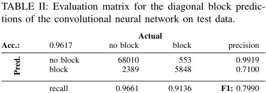
  特别地，这里准确度（precision）与召回率（recall）可以定义为：
  $$\begin{gathered} \mathrm{p}\mathrm{r}\mathrm{e}\mathrm{c}\mathrm{i}\mathrm{s}\mathrm{i}\mathrm{o}\mathrm{n}(y,\hat{y})=\frac{\mathrm{t}\mathrm{p}(y,\hat{y})}{\mathrm{t}\mathrm{p}(y,\hat{y})+\mathrm{f}\mathrm{p}(y,\hat{y})} \\ \mathrm{r}\mathrm{e}\mathrm{c}\mathrm{a}\mathrm{l}\mathrm{l}(y,\hat{y})=\frac{\mathrm{t}\mathrm{p}(y,\hat{y})}{\mathrm{t}\mathrm{p}(y,\hat{y})+\mathrm{f}\mathrm{n}(y,\hat{y})} \end{gathered}$$
  其中$y$是真实标签，$\hat{y}$是预测结果，$\mathrm{t}\mathrm{p},\mathrm{f}\mathrm{p},\mathrm{f}\mathrm{n}$即true positive rate，false positive rate与false negative rate；此外这两个值的调和平均即为$\mathrm{F}1$指标，不再赘述；

  无对角块的召回率相对于有对角块的召回率要高，模型在测试集的准确率高达$96.17\%$；

• 具体的模型评估结果见$\mathrm{T}\mathrm{a}\mathrm{b}\mathrm{l}\mathrm{e}3$与$\mathrm{T}\mathrm{a}\mathrm{b}\mathrm{l}\mathrm{e}4$：

  

  这个应该是关于判断矩阵是否存在对角块的一个分类的精确度，下面作者又对雅可比预条件子在GMRES迭代求解器中的实际效果做了一个验证，图像可见$\mathrm{F}\mathrm{i}\mathrm{g}\mathrm{u}\mathrm{r}\mathrm{e}8$

  

• 备注：

  这里最后总结一下，其实CNN并不只是预测某个矩阵是否存在对角块的表示（给定带宽$w$）的情况下，然后CNN还将能够把如何得到对角块的结果具体输出，上面的那个网络架构（$\mathrm{F}\mathrm{i}\mathrm{g}\mathrm{u}\mathrm{r}\mathrm{e}4$）可能需要好好研究一下，应该是个多输出的网络，具体还需要看代码，总之这个模型还挺有趣的，因为笔者最近的一次作业刚好与这个有点关系，之前确实一直没有看明白，现在做了作业再来看，感觉作业还有改进的地方，这里也稍微能看得明白一点了；

5 总结与展望 Summary and Outlook

We propose to employ machine learning techniques to generate preconditioner sparsity patterns. In this work, we have shown that a convolutional neural network can efficiently
detect strongly connected components in a matrix sparsity image, and that a therefrom derived block-Jacobi preconditioner is effective in accelerating the iterative solution process of the induced linear system. In future work, we plan to manually label a large set of test matrices taken from scientific applications which allows to move from artificially created test matrices to real-world problems. Furthermore, we will investigate the potential of using machine learning techniques for generating sparsity patterns for other problem-adapted preconditioners.

参考文献

[01] Mart´ın Abadi, Ashish Agarwal, Paul Barham, Eugene Brevdo, Zhifeng Chen, Craig Citro, Greg S. Corrado, Andy Davis, Jeffrey Dean, Matthieu Devin, Sanjay Ghemawat, Ian Goodfellow, Andrew Harp, Geoffrey Irving, Michael Isard, Yangqing Jia, Rafal Jozefowicz, Lukasz Kaiser, Manjunath Kudlur, Josh Levenberg, Dan Man´e, Rajat Monga, Sherry Moore, Derek Murray, Chris Olah, Mike Schuster, Jonathon Shlens, Benoit Steiner, Ilya Sutskever, Kunal Talwar, Paul Tucker, Vincent Vanhoucke, Vijay Vasudevan, Fernanda Vi´egas, Oriol Vinyals, Pete Warden, Martin Wattenberg, Martin Wicke, Yuan Yu, and Xiaoqiang Zheng. TensorFlow: Large-Scale Machine Learning on Heterogeneous Systems. arXiv preprint arXiv:1603.04467, 2015. [Online, Accessed: 2018-08-16 09:19 CEST]. 
[02] Jonas Adler and Ozan ¨Oktem. Solving ill-posed inverse problems using iterative deep neural networks. Inverse Problems, 33(12):124007, 2017. 
[03] Hartwig Anzt, Jack Dongarra, Goran Flegar, and Enrique S. QuintanaOrt´ı. Batched Gauss-Jordan elimination for block-Jacobi preconditioner generation on GPUs. In 8th Int. Workshop Programming Models & Appl. for Multicores & Manycores, PMAM, pages 1–10, 2017. 
[04] Hartwig Anzt, Jack Dongarra, Goran Flegar, and Enrique S. Quintana-Ort´ı. Variable-Size Batched LU for Small Matrices and Its Integration into Block-Jacobi Preconditioning. In 2017 46th International Conference on Parallel Processing (ICPP), pages 91–100, 2017. 
[05] Hartwig Anzt, Jack Dongarra, Goran Flegar, and Enrique S. Quintana-Ort´ı. Variable-size batched gauss–jordan elimination for block-jacobi preconditioning on graphics processors. Parallel Computing, 2018. 
[06] Hartwig Anzt, Jack Dongarra, Goran Flegar, Enrique S. Quintana-Ort´ı, and Andr´es E. Tom´as. Variable-Size Batched Gauss-Huard for Block-Jacobi Preconditioning. Procedia Computer Science, 108:1783 – 1792, 2017. International Conference on Computational Science, {ICCS} 2017, 12-14 June 2017, Zurich, Switzerland. 
[07] John Canny. A computational approach to edge detection. IEEE Transactions on pattern analysis and machine intelligence, (6):679–698, 1986. 
[08] Michael Chau and Hsinchun Chen. A machine learning approach to web page filtering using content and structure analysis. Decision Support Systems, 44(2):482 – 494, 2008. 
[09] Tianqi Chen, Mu Li, Yutian Li, Min Lin, Naiyan Wang, Minjie Wang, Tianjun Xiao, Bing Xu, Chiyuan Zhang, and Zheng Zhang. Mxnet: A flexible and efficient machine learning library for heterogeneous distributed systems. CoRR, abs/1512.01274, 2015. 
[10] Sharan Chetlur, Cliff Woolley, Philippe Vandermersch, Jonathan Cohen, John Tran, Bryan Catanzaro, and Evan Shelhamer. cudnn: Efficient primitives for deep learning. arXiv preprint arXiv:1410.0759, 2014. 
[11] Franc¸ois Chollet et al. Keras. https://github.com/fchollet/keras, 2015. [Online, Accessed: 2018-08-16 09:17 CEST]. 
[12] Edmond Chow, Hartwig Anzt, Jennifer Scott, and Jack Dongarra. Using jacobi iterations and blocking for solving sparse triangular systems in incomplete factorization preconditioning. Journal of Parallel and Distributed Computing, 119:219 – 230, 2018. 
[13] Andrew Collette. Python and HDF5. O’Reilly, 2013. ISBN: 978-1449367831. 
[14] Timothy Dozat. Incorporating Nesterov Momentum into Adam. 
[15] Lance B. Eliot. Advances in AI and Autonomous Vehicles: Cybernetic Self-Driving Cars Practical Advances in Artificial Intelligence (AI) and Machine Learning. LBE Press Publishing, 1st edition, 2017. 
[16] Markus G¨otz and Hartwig Anzt. Block prediction. https://github.com/ Markus-Goetz/block-prediction/, 2018. [Online, Accessed: 2018-08-28 09:95 CEST, Change set: 3f89d17]. 
[17] Kaiming He, Xiangyu Zhang, Shaoqing Ren, and Jian Sun. Identity mappings in deep residual networks. In European conference on computer vision, pages 630–645. Springer, 2016. 
[18] Markus Hegland and Paul E. Saylor. Block jacobi preconditioning of the conjugate gradient method on a vector processor. International Journal of Computer Mathematics, 44(1-4):71–89, 1992. 
[19] Norman P. et al. Jouppi. In-datacenter performance analysis of a tensor processing unit. SIGARCH Comput. Archit. News, 45(2):1–12, June 2017. 
[20] Diederik P Kingma and Jimmy Ba. Adam: A method for stochastic optimization. arXiv preprint arXiv:1412.6980, 2014. 
[21] G¨unter Klambauer, Thomas Unterthiner, Andreas Mayr, and Sepp Hochreiter. Self-normalizing neural networks. In Advances in Neural Information Processing Systems, pages 971–980, 2017. 
[22] Yann LeCun, Yoshua Bengio, and Geoffrey Hinton. Deep learning. nature, 521(7553):436, 2015. 
[23] Stefano Markidis, Steven Wei Der Chien, Erwin Laure, Ivy Bo Peng, and Jeffrey S. Vetter. NVIDIA tensor core programmability, performance & precision. CoRR, abs/1803.04014, 2018. 
[24] NVIDIA. NVIDIA CUDA TOOLKIT V9.0, March 2018. 
[25] NVIDIA Corp. Whitepaper: NVIDIA TESLA V100 GPU ARCHITECTURE, 2017. 
[26] Travis E Oliphant. A guide to NumPy, volume 1. Trelgol Publishing USA, 2006. 
[27] Adam Paszke, Sam Gross, Soumith Chintala, Gregory Chanan, Edward Yang, Zachary DeVito, Zeming Lin, Alban Desmaison, Luca Antiga, and Adam Lerer. Automatic differentiation in pytorch. 2017. 
[28] David Martin Powers. Evaluation: from precision, recall and f-measure to roc, informedness, markedness and correlation. 2011. 
[29] J¨urgen Schmidhuber. Deep learning in neural networks: An overview. Neural Networks, 61:85 – 117, 2015. 
[30] Nitish Srivastava, Geoffrey Hinton, Alex Krizhevsky, Ilya Sutskever, and Ruslan Salakhutdinov. Dropout: a simple way to prevent neural networks from overfitting. The Journal of Machine Learning Research, 15(1):1929–1958, 2014. 
[31] W. Tang, T. Shan, X. Dang, M. Li, F. Yang, S. Xu, and J. Wu. Study on a poisson’s equation solver based on deep learning technique. In 2017 IEEE Electrical Design of Advanced Packaging and Systems Symposium (EDAPS), pages 1–3, Dec 2017. 
[32] Yue Zhao, Jiajia Li, Chunhua Liao, and Xipeng Shen. Bridging the gap between deep learning and sparse matrix format selection. SIGPLAN Not., 53(1):94–108, February 2018. 

图表汇总