线性回归波士顿房价预测

线性回归对波士顿房价进行预测主要从以下八个方面来对本次内容进行实验。序号任务名称任务具体要求1数据理解理解数据集背景以及数据含义。2数据读入使用pandas 读入数据并输出读入的数据3定义特征值，目标值使用'crim', 'rm', 'l

文章共4,448字 · 阅读需要大约15分钟

一键AI生成摘要，助你高效阅读

问答

bit_100

30499人浏览 · 2021-05-02 22:21:57

bit_100 · 2021-05-02 22:21:57 发布

线性回归对波士顿房价进行预测

一、基础概念：

1. 线性回归

回归分析，数理统计学中，回归分析着重在寻求变量之间近似的函数关系。

线性回归分析，就是寻求变量之间近似的线性函数关系。

线性回归就是回归函数为线性函数的情形。

2. 平均绝对误差，均方误差的理解

平均绝对误差（MAE）是一种线性分数，所有个体差异在平均值上的权重都相等。表示预测值和观测值之间绝对误差的平均值。

均方误差（MSE）即方差，MSE表示预测数据和原始数据对应点误差的平方和的均值。

，其中n为样本的个数。

线性回归中，MSE（L2损失）计算简便，但MAE（L1损失）对异常点有更好的鲁棒性。当预测值和真实值接近时，误差的方差较小；反之误差方差非常大，相比于MAE，使用MSE会导致异常点有更大的权重，因此数据有异常点时，使用MAE损失函数更好。

3. 决定系数 $R^{2}$

利用决定系数 $R^{2}$ 来量化本次实验中的线性回归模型的表现，表示的是目标变量的预测值和实际值之间的相关程度平方的百分比。决定系数为1的模型表示可以对目标变量进行完美的预测；为0时则很难预测，换用其他标准预测；在0到1之间则表示模型中目标变量有百分之多少可以由选定的特征值来预测。

二、实验步骤与分析

主要从以下八个方面来对本次内容进行实验。

序号	任务名称	任务具体要求
1	数据理解	理解数据集背景以及数据含义。
2	数据读入	使用pandas 读入数据并输出读入的数据
3	定义特征值，目标值	使用'crim', 'rm', 'lstat'作为特征值，'medv'为目标值，输出特征值的描述性统计
4	区分训练集和测试集	split_num = int(len(features)*0.7)
5	线性回归	利用sklearn的LinearRegression()函数进行线性回归，输出模型的回归方程系数及方程的截距
6	预测	对数据集进行预测，输出预测值
7	获取平均绝对误差	求取预测值和真实值的mae
8	获取均分误差	求取预测值和真实值的mse

1. 数据背景

2. 数据读入

boston = datasets.load_boston()
print(boston)

boston_df = pd.DataFrame(boston.data, columns=boston.feature_names)
boston_df['MEDV'] = boston.target

# 查看数据是否存在空值，从结果来看数据不存在空值。
boston_df.isnull().sum()
# 查看数据大小
boston_df.shape
# 显示数据前5行
boston_df.head()

# 查看数据的描述信息，在描述信息里可以看到每个特征的均值，最大值，最小值等信息。
boston_df.describe()
# 各个特征和MEDV的线性关系。
plt.figure(facecolor='gray')
corr = boston_df.corr()
corr = corr['MEDV']
corr[abs(corr) > 0.5].sort_values().plot.bar()

如上图所示，LSTAT、PTRATIO、RM和MEDV的相关性都超过0.5。

接下来通过数据分布图来观察特征值'crim', 'rm', 'lstat'和目标值'medv'之间的关系。

# LSTAT 和MEDV的散点图
plt.figure(facecolor='gray')
plt.scatter(boston_df['LSTAT'], boston_df['MEDV'], s=30, edgecolor='white')
plt.title('LSTAT')

通过上图可以得出：低收入人群占比越高，MEDV即同类房价中位数越低。

# CRIM 和MEDV的散点图
plt.figure(facecolor='gray')
plt.scatter(boston_df['CRIM'], boston_df['MEDV'], s=30, edgecolor='white')
plt.title('CRIM')

通过上图得出：犯罪率越高，房价中位数越低。

# RM 和MEDV的散点图
plt.figure(facecolor='gray')
plt.scatter(boston_df['RM'], boston_df['MEDV'], s=30, edgecolor='white')
plt.title('RM')
plt.show()

右上图可知：屋房间数越多，房屋价格中位数普遍越高。

3. 定义特征值、目标值

#分析房屋的’RM’， ‘LSTAT’，'CRIM’ 特征与MEDV的相关性性，所以，将其余不相关特征移除
boston_df = boston_df[['LSTAT', 'CRIM', 'RM', 'MEDV']]
# 目标值
y = np.array(boston_df['MEDV'])
boston_df = boston_df.drop(['MEDV'], axis=1)
# 特征值
X = np.array(boston_df)

4. 区分训练集和测试集

from sklearn.model_selection import train_test_split

#70%用于训练，30%用于测试
X_train, X_test, y_train, y_test = train_test_split(X, y, test_size=0.3, random_state=10)
print(X_train.shape, X_test.shape, y_train.shape, y_test.shape)

5. 线性回归

#线性回归
from sklearn.linear_model import LinearRegression
lr = LinearRegression()
# 使用训练数据进行参数估计
lr.fit(X_train, y_train)

# 输出线性回归的系数
print('线性回归的系数为:\n w = %s \n b = %s' % (lr.coef_, lr.intercept_))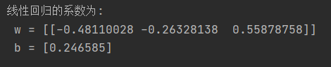

6. 进行预测

# 使用测试数据进行回归预测
	y_test_pred = lr.predict(X_test)
	print('y_test_pred : ', y_test_pred)

7. 获取平均值

#计算平均绝对误差
	train_MAE = [mean_absolute_error(y_train, [np.mean(y_train)] * len(y_train)),
               mean_absolute_error(y_train, y_train_pred)]

8. 获取均分绝对误差

# 计算均分方差
	train_MSE = [mean_squared_error(y_train, [np.mean(y_train)] * len(y_train)),
               mean_squared_error(y_train, y_train_pred)]

通过决定系数 $R^{2}$ 量化分析模型的表现。

如上图，该线性回归模型的决定系数为0.4531，即该模型中目标变量有45.31%可以用特征来解释，说明线性关系可以解释同类房价中位数（MEDV）的45.31% 。

完整代码：

import numpy as np
import pandas as pd
import matplotlib.pyplot as plt
import seaborn as sns
from sklearn import datasets
# 加载波士顿房价的数据集
#boston = pd.read_csv('boston.csv')
boston = datasets.load_boston()
print(boston)

boston_df = pd.DataFrame(boston.data, columns=boston.feature_names)
boston_df['MEDV'] = boston.target

# 查看数据是否存在空值，从结果来看数据不存在空值。
boston_df.isnull().sum()
# 查看数据大小
boston_df.shape
# 显示数据前5行
boston_df.head()

# 查看数据的描述信息，在描述信息里可以看到每个特征的均值，最大值，最小值等信息。
boston_df.describe()
#
# # 清洗'PRICE' = 50.0 的数据
# boston_df = boston_df.loc[boston_df['PRICE'] != 50.0]

# 计算每一个特征和房价的相关系数
boston_df.corr()['MEDV']


# 各个特征和价格都有明显的线性关系。
plt.figure(facecolor='gray')
corr = boston_df.corr()
corr = corr['MEDV']
corr[abs(corr) > 0.5].sort_values().plot.bar()

# LSTAT 和房价的散点图
plt.figure(facecolor='gray')
plt.scatter(boston_df['LSTAT'], boston_df['MEDV'], s=30, edgecolor='white')
plt.title('LSTAT')
plt.xlabel('LSTAT')
plt.ylabel('MEDV')

# CRIM 和房价的散点图
plt.figure(facecolor='gray')
plt.scatter(boston_df['CRIM'], boston_df['MEDV'], s=30, edgecolor='white')
plt.title('CRIM')
plt.xlabel('CRIM')
plt.ylabel('MEDV')

# RM 和房价的散点图
plt.figure(facecolor='gray')
plt.scatter(boston_df['RM'], boston_df['MEDV'], s=30, edgecolor='white')
plt.title('RM')
plt.xlabel('RM')
plt.ylabel('MEDV')
plt.show()

boston_df = boston_df[['LSTAT', 'CRIM', 'RM', 'MEDV']]
# 目标值
y = np.array(boston_df['MEDV'])
boston_df = boston_df.drop(['MEDV'], axis=1)
# 特征值
X = np.array(boston_df)

from sklearn.model_selection import train_test_split
X_train, X_test, y_train, y_test = train_test_split(X, y, test_size=0.3, random_state=10)
print(X_train.shape, X_test.shape, y_train.shape, y_test.shape)

from sklearn import preprocessing
# 初始化标准化器
min_max_scaler = preprocessing.MinMaxScaler()
# 分别对训练和测试数据的特征以及目标值进行标准化处理
X_train = min_max_scaler.fit_transform(X_train)
y_train = min_max_scaler.fit_transform(y_train.reshape(-1,1)) # reshape(-1,1)指将它转化为1列，行自动确定
X_test = min_max_scaler.fit_transform(X_test)
y_test = min_max_scaler.fit_transform(y_test.reshape(-1,1))

from sklearn.linear_model import LinearRegression
lr = LinearRegression()
# 使用训练数据进行参数估计
lr.fit(X_train, y_train)
# 使用测试数据进行回归预测
y_test_pred = lr.predict(X_test)
print('y_test_pred : ', y_test_pred)

# 使用r2_score对模型评估
from sklearn.metrics import mean_squared_error, mean_absolute_error, r2_score

# 绘图函数
def figure(title, *datalist):
    plt.figure(facecolor='gray', figsize=[16, 8])
    for v in datalist:
        plt.plot(v[0], '-', label=v[1], linewidth=2)
        plt.plot(v[0], 'o')
    plt.grid()
    plt.title(title, fontsize=20)
    plt.legend(fontsize=16)
    plt.show()

# 训练数据的预测值
y_train_pred = lr.predict(X_train)
print('y_train_pred : ', y_train_pred)
# 计算均分方差
train_MSE = [mean_squared_error(y_train, [np.mean(y_train)] * len(y_train)),
               mean_squared_error(y_train, y_train_pred)]

#计算平均绝对误差
train_MAE = [mean_absolute_error(y_train, [np.mean(y_train)] * len(y_train)),
               mean_absolute_error(y_train, y_train_pred)]


# 绘制误差图
figure(' MSE = %.4f' % (train_MSE[-1]), [train_MSE, 'MSE'])
figure(' MAE = %.4f' % (train_MAE[-1]), [train_MAE, 'MAE'])


# 绘制预测值与真实值图
figure('预测值与真实值图 模型的' + r'$R^2=%.4f$' % (r2_score(y_train_pred, y_train)), [y_test_pred, 'pred_value'],
       [y_test, 'true_value'])
# 线性回归的系数
print('线性回归的系数为:\n w = %s \n b = %s' % (lr.coef_, lr.intercept_))