张量的概念及基本运算

1 张量的定义

  张量是一个多维数组。更正式地说，一个 N 阶张量是 N 个向量空间元素的张量积，每个向量空间都有自己的坐标系。
  张量的阶数（the order of a tensor）也称为维数（dimensions）、模态（modes）、或方式（ways）。

一阶张量是一个矢量，二阶张量是一个矩阵，三阶或更高阶的张量叫做高阶张量。

2 纤维（Fibers）与 切片（Slices）

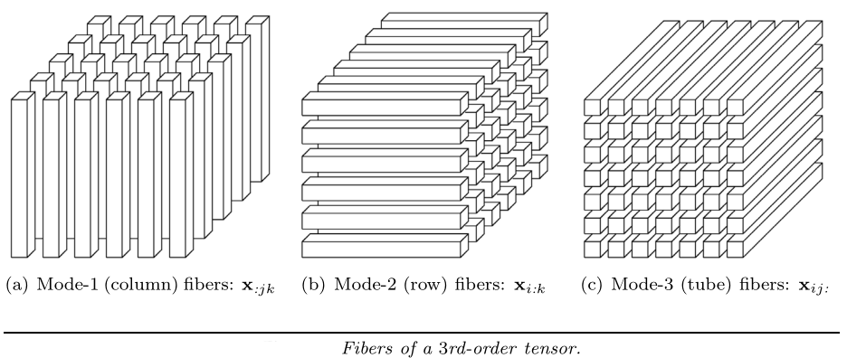
2.1 纤维（Fibers）

纤维(Fibers) 是矩阵的行和列的高阶类似物。（纤维是指从张量中抽取的向量）
例如，矩阵 A 的列为mode-1纤维，行为mode-2纤维；

三阶张量有 列(column) 、行(row) 、管(tube) 纤维，分别用${\mathbf{x}}_{:,j,k}$ , ${\mathbf{x}}_{i,:,k}$ , ${\mathbf{x}}_{i,j,:}$ 表示。

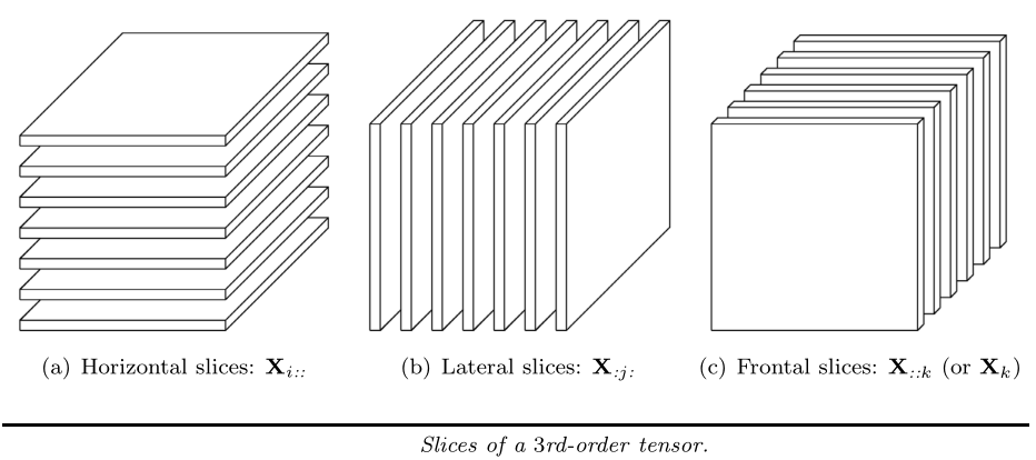
2.2 切片（Slices）

切片 (Slices) 是一个张量的二维切片，通过固定除两个维度之外的索引来定义。（切片是指从张量中抽取的矩阵）

• 例如，三阶张量 $\mathcal{X}$ 的 水平面(horizontal) 、 侧面(lateral) 和 正面(frontal) 的切片，分别用 ${\mathbf{X}}_{i,:,:}$ , ${\mathbf{X}}_{:,j,:}$ 和 ${\mathbf{X}}_{:,:,k}$ 表示，且 ${\mathbf{X}}_{:,:,k}$ 可简记为 ${\mathbf{X}}_k$

3 张量的范数（norm）

张量 $\mathcal{X}\in {\mathbb{R}}^{I_1\times I_2\times \cdots \times I_N}$ 的范数是其所有元素平方和的平方根，即:
$$\Vert \mathcal{X}\Vert =\sqrt{\sum _{i_1=1}^{I_1}\sum _{i_2=1}^{I_2}\cdots \sum _{i_N=1}^{I_N}{x}_{i_1{i}_2\cdots i_N}^2}$$
这类似于矩阵 $\mathbf{A}$ 的 F范数(Frobenius norm).

4 张量的内积（inner product）

两个相同大小张量 $\mathcal{X},\mathcal{Y}\in {\mathbb{R}}^{I_1\times I_2\times \cdots \times I_N}$ 的内积，即
$$⟨\mathcal{X},\mathcal{Y}⟩=\sum _{i_1=1}^{I_1}\sum _{i_2=1}^{I_2}\cdots \sum _{i_N=1}^{I_N}{x}_{i_1{i}_2\cdots i_N}{y}_{i_1{i}_2\cdots i_N}$$
且有
$$⟨\mathcal{X},\mathcal{X}⟩=\Vert \mathcal{X}{\Vert }^2$$

5 秩1张量（Rank-One Tensors）

一个 N 维张量 $\mathcal{X}\in {\mathbb{R}}^{I_1\times I_2\times \cdots \times I_N}$ ，如果可以被写成 N 个向量的张量外积(outer product) ，
$$\mathcal{X}={\mathbf{a}}^{(1)}\circ {\mathbf{a}}^{(2)}\circ \cdots \circ {\mathbf{a}}^{(N)}$$
则这个张量的秩为1.

其中，符号“◦”代表张量外积，即，张量的每个元素都是对应的向量元素的乘积：
$$x_{i_1{i}_2\cdots i_N}=a_{i_1}^{(1)}{a}_{i_2}^{(2)}\cdots a_{i_N}^{(N)}\text{ for all }1\le i_n\le I_n$$
下图展示了 $\mathcal{X}=a\circ b\circ c$，一个三阶秩1张量

• 注：
  ① 张量外积（Outer Product） 是线性代数中的外积， 也就是张量积（Tensor Product）；克罗内克积（Kronecker Product）是张量积在矩阵中的特殊形式。
  ② 向量外积（Exterior Product） 是解析几何中的外积，也叫叉积（Cross Product）。

6 对称性与张量（Symmetry and Tensors）

6.1 立方张量（cubical tensors）

如果一个张量的每个维度大小相同，$\mathcal{X}\in {\mathbb{R}}^{I\times I\times I\times \cdots \times I}$，那么这个张量就叫做立方（cubical）张量；

6.2 超对称张量（super symmetric）

如果立方张量在任何索引排列下都保持不变，则立方张量称为超对称张量（supersymmetric）（或对称张量）。

• 例如，如果满足以下条件，则三阶张量 $\mathcal{X}\in {\mathbb{R}}^{I\times I\times I}$ 是超对称的
  $$x_{ijk}=x_{ikj}=x_{jik}=x_{jki}=x_{kij}=x_{kji}\text{ for all }i,j,k=1,\dots ,I$$

6.3 部分对称张量（partically symmetric）

张量也可在两个或多个维度下(部分)对称。

• 例如，对于三阶张量 $\mathcal{X}\in {\mathbb{R}}^{I\times I\times K}$ ，如果所有的正面切片都是对称的，
  $${\mathbf{X}}_k={\mathbf{X}}_k^{\top }\text{ for all }k=1,\dots ,K$$
  则该三阶张量在mode-1 和 mode-2 下是对称的。

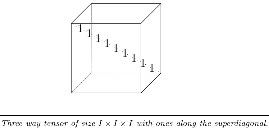
7 对角张量（Diagonal Tensors）

如果一个张量 $\mathcal{X}\in {\mathbb{R}}^{I_1\times I_2\times \cdots \times I_N}$ ，当且仅当 $x_{i_1{i}_2\cdots i_N}\ne 0$ 时，有 $i_1=i_2=\cdots =i_N$ ，则该张量是对角（diagonal）张量。
下图展示了一个沿超对角线分布的立方张量。

8 矩阵化：将张量转化为矩阵（Matricization: Transforming a Tensor into a Matrix）

矩阵化(Matricization)，也就是所谓的“展开”(unfolding)或“压扁”(flattening)，是将一个 n 维数组中的元素重新排列成一个矩阵的过程。

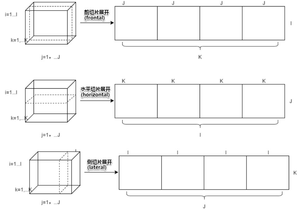
• 例如，一个2×3×4张量可以被重排成一个 6×4 或 3×8 的矩阵等。

张量 $\mathcal{X}\in {\mathbb{R}}^{I_1\times I_2\times \cdots \times I_N}$ 的 mod-n 矩阵化记为 ${\mathbf{X}}_{(n)}$ ,它是将第 n 维纤维作为结果矩阵的列。即将张量元素 $\left(i_1,i_2,\dots ,i_N\right)$ 映射到矩阵元素 $\left(i_n,j\right)$ 中
$$j=1+\sum _{\genfrac{}{}{0ex}{}{k=1}{k\ne n}}^N\left(i_k-1\right)J_k\text{ with }{J}_k=\prod _{\genfrac{}{}{0ex}{}{m=1}{m\ne n}}^{k-1}{I}_m$$

• 例，设张量 $x\in {\mathbb{R}}^{3\times 4\times 2}$ 的前切片为：
  $${\mathbf{X}}_1=\left[\begin{array}{llll}1& 4& 7& 10\\ 2& 5& 8& 11\\ 3& 6& 9& 12\end{array}\right],{\mathbf{X}}_2=\left[\begin{array}{llll}13& 16& 19& 22\\ 14& 17& 20& 23\\ 15& 18& 21& 24\end{array}\right]$$

则三个mode-n的展开分别是

$$\begin{array}{rl}{\mathbf{X}}_{(1)}& =\left[\begin{array}{llllllll}1& 4& 7& 10& 13& 16& 19& 22\\ 2& 5& 8& 11& 14& 17& 20& 23\\ 3& 6& 9& 12& 15& 18& 21& 24\end{array}\right]\\ {\mathbf{X}}_{(2)}& =\left[\begin{array}{cccccc}1& 2& 3& 13& 14& 15\\ 4& 5& 6& 16& 17& 18\\ 7& 8& 9& 19& 20& 21\\ 10& 11& 12& 22& 23& 24\end{array}\right]\\ {\mathbf{X}}_{(3)}& =\left[\begin{array}{cccccccccc}1& 2& 3& 4& 5& \cdots & 9& 10& 11& 12\\ 13& 14& 15& 16& 17& \cdots & 21& 22& 23& 24\end{array}\right]\end{array}$$

最后，向量化一个张量也是可以。同样，只要元素的顺序是一致的，它就不重要。在上面的例子中，向量化的版本是：
$$\mathrm{vec}(\mathbf{X})=\left[\begin{array}{c}1\\ 2\\ ⋮\\ 24\end{array}\right]$$

9 张量乘积：n模乘（Tensor Multiplication : The n-Mode Product）

张量可以相乘，尽管显然它的符号和符号要比矩阵复杂得多。对于张量乘法的完整处理参见：Bader, MATLAB Tensor Classes forFast Algorithm Prototyping,2006.
这里我们只考虑张量n模乘（n-mode product），即用一个张量乘以一个n维矩阵(或向量)。

9.1 n模矩阵积（n-mode matrix product）

（1）定义
张量 $\mathcal{X}\in {\mathbb{R}}^{I_1\times I_2\times \cdots \times I_N}$ 与矩阵 $\mathbf{U}\in {\mathbb{R}}^{J\times I_n}$ 的n模（矩阵）积记为 $\mathcal{X}{\times }_n\mathbf{U}$ ，尺寸为 $I_1\times \cdots \times I_{n-1}\times J\times I_{n+1}\times \cdots \times I_N$ 。从元素上看有：

$${\left(\mathcal{X}{\times }_n\mathbf{U}\right)}_{i_1\cdots i_{n-1}j{i}_{n+1}\cdots i_N}=\sum _{i_n=1}^{I_n}{x}_{i_1{i}_2\cdots i_N}{u}_{j{i}_n}$$

即每个n模纤维都乘以矩阵$\mathbf{U}$。这个想法也可以用矩阵化张量表示：
$$\mathcal{Y}=\mathcal{X}{\times }_n\mathbf{U}\iff {\mathbf{Y}}_{(n)}={\mathbf{U}\mathbf{X}}_{(n)}$$

（2）例题
设张量 $x\in {\mathbb{R}}^{3\times 4\times 2}$ 的前切片为：
$${\mathbf{X}}_1=\left[\begin{array}{llll}1& 4& 7& 10\\ 2& 5& 8& 11\\ 3& 6& 9& 12\end{array}\right],{\mathbf{X}}_2=\left[\begin{array}{llll}13& 16& 19& 22\\ 14& 17& 20& 23\\ 15& 18& 21& 24\end{array}\right]$$
矩阵：$\mathbf{U}=\left[\begin{array}{ccc}1& 3& 5\\ 2& 4& 6\end{array}\right]$
则张量与矩阵的1模乘为：
$$\mathcal{Y}=\mathcal{X}{\times }_1\mathbf{U}\in {\mathbb{R}}^{2\times 4\times 2}$$
其中，
$${\mathbf{Y}}_1=\left[\begin{array}{cccc}22& 49& 76& 103\\ 28& 64& 100& 136\end{array}\right],{\mathbf{Y}}_2=\left[\begin{array}{cccc}130& 157& 184& 211\\ 172& 208& 244& 280\end{array}\right]$$

（3）基本运算法则
① 连模乘
对于一系列乘法中的不同mode，乘法的顺序是不相关的，即
$$\mathcal{X}{\times }_m\mathbf{A}{\times }_n\mathbf{B}=\mathcal{X}{\times }_n\mathbf{B}{\times }_m\mathbf{A}(m\ne n)$$
如果mode相同，则
$$\mathcal{X}{\times }_n\mathbf{A}{\times }_n\mathbf{B}=\mathcal{X}{\times }_n\left(\mathbf{B}\mathbf{A}\right)$$

② 特殊地，矩阵情形为：
$$\mathbf{A}\mathbf{B}\mathbf{C}=\mathbf{B}{\times }_1\mathbf{A}{\times }_2{\mathbf{C}}^{\mathrm{T}}$$

$${\mathbf{x}}^{\mathrm{T}}\mathbf{A}\mathbf{y}=\mathbf{A}{\times }_1{\mathbf{x}}^{\mathrm{T}}{\times }_2{\mathbf{y}}^{\mathrm{T}}=\mathbf{A}{\times }_1\mathbf{x}{\times }_2\mathbf{y}$$

9.2 n模向量积（The n-mode vector product）

（1）定义
张量 $\mathcal{X}\in {\mathbb{R}}^{I_1\times I_2\times \cdots \times I_N}$ 与向量 $\mathbf{v}\in {\mathbb{R}}^{I_n}$ 的n模（向量）积记为 $\mathcal{X}{\overline{\times }}_n\mathbf{v}$ ，尺寸为 $I_1\times \cdots \times I_{n-1}\times I_{n+1}\times \cdots \times I_N$ 。从元素上看有：
$${\left(\mathcal{X}{\overline{\times }}_n\mathbf{v}\right)}_{i_1\cdots i_{n-1}{i}_{n+1}\cdots i_N}=\sum _{i_n=1}^{I_n}{x}_{i_1{i}_2\cdots i_N}{v}_{i_n}$$
（2）例题
设张量 $x\in {\mathbb{R}}^{3\times 4\times 2}$ 的前切片为：
$${\mathbf{X}}_1=\left[\begin{array}{llll}1& 4& 7& 10\\ 2& 5& 8& 11\\ 3& 6& 9& 12\end{array}\right],{\mathbf{X}}_2=\left[\begin{array}{llll}13& 16& 19& 22\\ 14& 17& 20& 23\\ 15& 18& 21& 24\end{array}\right]$$
向量：$\mathbf{v}={\left[\begin{array}{cccc}1& 2& 3& 4\end{array}\right]}^T$
则张量与向量的2模乘为：
$$\mathcal{X}{\overline{\times }}_2\mathbf{v}=\left[\begin{array}{cc}70& 190\\ 80& 200\\ 90& 210\end{array}\right]$$

（3）基本运算法则
当涉及到模n向量乘法时，优先级很重要，因为中间结果的顺序会改变。即
$$\mathcal{X}{\overline{\times }}_m\mathbf{a}{\overline{\times }}_n\mathbf{b}=\left(\mathcal{X}{\overline{\times }}_m\mathbf{a}\right){\overline{\times }}_{n-1}\mathbf{b}=\left(\mathcal{X}{\overline{\times }}_n\mathbf{b}\right){\overline{\times }}_m\mathbf{a}\text{ for }m<n$$

10 矩阵Kronecker积、Khatri–Rao积与Hadamard积

10.1 Kronecker积

矩阵 $\mathbf{A}\in {\mathbb{R}}^{I\times J}$ 与 $\mathbf{B}\in {\mathbb{R}}^{K\times L}$ 的 Kronecker 积记为 $\mathbf{A}\otimes \mathbf{B}$ ，其结果大小为 $(IK)\times (JL)$ 的矩阵：

$$\begin{array}{rl}\mathbf{A}\otimes \mathbf{B}& =\left[\begin{array}{cccc}{a}_{11}\mathbf{B}& a_{12}\mathbf{B}& \cdots & a_{1J}\mathbf{B}\\ a_{21}\mathbf{B}& a_{22}\mathbf{B}& \cdots & a_{2J}\mathbf{B}\\ ⋮& ⋮& \ddots & ⋮\\ a_{I1}\mathbf{B}& a_{I2}\mathbf{B}& \cdots & a_{IJ}\mathbf{B}\end{array}\right]\\ & =\left[{\mathbf{a}}_1\otimes {\mathbf{b}}_1{\mathbf{a}}_1\otimes {\mathbf{b}}_2{\mathbf{a}}_1\otimes {\mathbf{b}}_3\cdots {\mathbf{a}}_J\otimes {\mathbf{b}}_{L-1}{\mathbf{a}}_J\otimes {\mathbf{b}}_L\right]\end{array}$$

10.2 Khatri–Rao积

Khatri–Rao积是Kronecker积的“matching columnwise”
矩阵 $\mathbf{A}\in {\mathbb{R}}^{I\times K}$ 与 $\mathbf{B}\in {\mathbb{R}}^{J\times K}$ 的 Khatri–Rao 积记为 $\mathbf{A}\otimes \mathbf{B}$ ，其结果大小为 $(IJ)\times K$ 的矩阵：

$$\mathbf{A}\odot \mathbf{B}=\left[\begin{array}{llll}{\mathbf{a}}_1\otimes {\mathbf{b}}_1& {\mathbf{a}}_2\otimes {\mathbf{b}}_2& \cdots & {\mathbf{a}}_K\otimes {\mathbf{b}}_K\end{array}\right]$$

向量的Kronecker积与Khatri-Rao积相等：
$$\mathbf{a}\otimes \mathbf{b}=\mathbf{a}\odot \mathbf{b}$$

10.3 Hadamard积

Hadamard积是矩阵的元素积（按元素点乘）
矩阵$\mathbf{A}$和$\mathbf{B}$尺寸均为$I\times J$，它们的Hadamard积记为$\mathbf{A}\ast \mathbf{B}$，其结果为大小$I\times J$的矩阵

$$\mathbf{A}\ast \mathbf{B}=\left[\begin{array}{cccc}{a}_{11}{b}_{11}& a_{12}{b}_{12}& \cdots & a_{1J}{b}_{1J}\\ a_{21}{b}_{21}& a_{22}{b}_{22}& \cdots & a_{2J}{b}_{2J}\\ ⋮& ⋮& \ddots & ⋮\\ a_{I1}{b}_{I1}& a_{I2}{b}_{I2}& \cdots & a_{IJ}{b}_{IJ}\end{array}\right]$$

10.4 性质

上面讨论的各种积，有如下性质：
$$\begin{array}{rl}(\mathbf{A}\otimes \mathbf{B})(\mathbf{C}\otimes \mathbf{D})& =\mathbf{A}\mathbf{C}\otimes \mathbf{B}\mathbf{D}\\ (\mathbf{A}\otimes \mathbf{B}{)}^{†}& ={\mathbf{A}}^{†}\otimes {\mathbf{B}}^{†}\\ \mathbf{A}\odot \mathbf{B}\odot \mathbf{C}& =(\mathbf{A}\odot \mathbf{B})\odot \mathbf{C}=\mathbf{A}\odot (\mathbf{B}\odot \mathbf{C})\\ (\mathbf{A}\odot \mathbf{B}{)}^{\top }(\mathbf{A}\odot \mathbf{B})& ={\mathbf{A}}^{\top }\mathbf{A}\ast {\mathbf{B}}^{\top }\mathbf{B}\\ (\mathbf{A}\odot \mathbf{B}{)}^{†}& ={\left(\left({\mathbf{A}}^{\top }\mathbf{A}\right)\ast \left({\mathbf{B}}^{\top }\mathbf{B}\right)\right)}^{†}(\mathbf{A}\odot \mathbf{B}{)}^{\top }\end{array}$$

其中，${\mathbf{A}}^{†}$ 为 $\mathbf{A}$ 的Moore-Penrose伪逆。

---

参考文献：
[1] Kolda T G , Bader B W . Tensor Decompositions and Applications[J]. SIAM Review, 2009, 51(3):455-500.