
深度学习入门
·
理论知识
Q1. 神经网络训练过程中,哪些量是已知的,哪些量是未知的?学习的目标到底是什么?
A1.已知:训练数据(输入和标签),测试数据(对模型来说x已知y不已知),损失函数;未知:神经网路的权重和偏置。
学习的目标是让机器从训练数据中总结规律,找到一组权重和偏置,让损失函数的值更小,模型的预测结果更符合真实值。
Q2. 为什么单层感知机只能解决线性可分问题?
A2.因为单层感知机的公式为y=h(b+w1x1+w2y2),训练时不断调整w和b,所以b+w1x1+w2y2部分为一条直线,只能解决线性可分问题。
Q3. 为什么必须引入非线性激活函数? 如果把神经网络中所有激活函数都去掉,会发生什么?
A3.如果不引用非线性激活函数,那么神经网络不管层数有多少,多层线性都会有与之等价的一层线性。
Q4. 神经网络的前向传播,本质上在做什么数学运算?
A4.是在做激活函数和线性函数的组合运算。
Q5. 为什么分类问题中,输出层通常使用 Softmax? Softmax 在概率意义上做了什么?
A5.因为分类问题如果没有softmax,得到的结果将是一堆实数,不方便人们观察。而softmax将这些有正有负有大有小的实数都转化为对应的概率,且这些概率相加为1,更直观。
Q6. 为什么“准确率”不能作为训练时的优化目标? 为什么必须引入损失函数?
A6.因为如果使用准确率作为指标,在权重改动较小时大多数地方的导数都会变为0,无法知道更新方向。而引入损失函数后权重的改动都会带来损失函数导数的变化,从而能改动使其值变小,进而间接提高准确率。
Q7. 梯度在几何意义上代表什么? 为什么沿着负梯度方向更新参数?
A7.梯度是一个向量,指向函数在该点上升最快的方向,而其大小是此时的变化率。所以负梯度方向就是函数下降最快的方向。沿着负梯度方向更新参数是为了损失函数下降,从而提升准确率。
Q8. 学习率在梯度下降中起什么作用? 学习率过大会怎样? 过小又会怎样?
A8.学习率决定了在一次学习中,应该学习多少,以及在多大程度上更新参数,过小会使训练低效,更新缓慢,过大会使训练太发散,可能更新过头,不够稳定。
手写神经网络与手写数字实践
激活函数
import numpy as np

#常用于二分类问题输出层,压缩输出值为0到1
def sigmoid(x):
    return 1/(1+np.exp(-x))

#常用于神经网路的隐藏层,环节梯度消失问题
def relu(x):
    return np.maxinum(0,x)

#常用于多分类且类别相互排斥问题的隐藏层,压缩输出值为0到1
def softmax(x):
    c=np.max(a)
    exp_a=np.exp(a-c)
    sum_exp_p=np.sum(exp_a)
    y=exp_a/sum_exp_a
    return y
损失函数
#交叉熵误差
#t为独热编码数组
#单组数据
def cross_entropy_error(y,t):
    delta = 1e-7
    return -np.sum(t*np.log(y + delta))

#支持batch输入
def cross_entropy_error(y,t):
    if y.ndim == 1:
        t = t.reshape(1,t.size)
        y = y.reshape(1,y.size)
    batch_size = y.shape[0]
    return -np.sum(t*np.log(y + 1e-7))/batch_size

#t为标签形式
def cross_entropy_error(y,t):
    if y.ndim == 1
        t = t.reshape(1,t.size)
        y = y.reshape(1,y.size)
    batch_size = y.shape[0]
    return -np.sum(np.log(y[np.arrange(batch_size),t]+1e-7))/batch_size
数值梯度
def numerical_gradient(f, x):#x为Numpy数组,f为函数
    h = 1e-4 # 0.0001
    grad = np.zeros_like(x) # 生成和x形状相同的所有元素为0的数组
    for idx in range(x.size):
        tmp_val = x[idx]
        # f(x+h)的计算
        x[idx] = tmp_val + h
        fxh1 = f(x)

        # f(x-h)的计算
        x[idx] = tmp_val - h
        fxh2 = f(x)

        grad[idx] = (fxh1 - fxh2) / (2*h)
        x[idx] = tmp_val # 还原值
	return grad
#这样生成的就是所有x变量的偏导数的数组了
实现神经网络
import numpy as np
import matplotlib.pyplot as plt
from sklearn.datasets import fetch_openml

#下载数据
mnist = fetch_openml('mnist_784',version=1,as_frame=False)
#切分数据
x, y = mnist.data, mnist.target.astype(np.uint8)
x_train, x_test = x[:5000], x[2000:]
y_train, y_test = y[:5000], y[2000:]
#数据归一化
x_train = x_train.astype(np.float32) / 255.0
x_test = x_test.astype(np.float32) / 255.0


print(f'训练集图像形状: {x_train.shape}, 标签数量: {len(y_train)}')
print(f'测试集图像形状: {x_test.shape}, 标签数量: {len(y_test)}')

#生成梯度
def numerical_gradient(f,x):
    h = 1e-4
    x_flat = x.flatten()
    grad_flat = np.zeros_like(x_flat)
    for idx in range(x_flat.size):
        tmp_val = x_flat[idx]
        x_flat[idx] = tmp_val + h
        x_new = x_flat.reshape(x.shape)  # 还原为原形状
        fxh1 = f(x_new)
        x_flat[idx] = tmp_val - h
        x_new = x_flat.reshape(x.shape)
        fxh2 = f(x_new)
        grad_flat[idx] = (fxh1 - fxh2)/(2*h)
        x_flat[idx] = tmp_val

        grad = grad_flat.reshape(x.shape)
    return grad

#梯度下降法
def gradient_descent(f,init_x,lr=0.01,step_num=100):
    x = init_x
    for i in range(step_num):
        grad = numerical_gradient(f,x)
        x -= lr*grad
    return x

#激活函数
def relu(x):
    return np.maximum(0,x)

def softmax(a):
    c = np.max(a,axis=-1, keepdims=True)
    exp_a = np.exp(a-c)
    sum_exp_a = np.sum(exp_a,axis=-1, keepdims=True)
    y = exp_a / sum_exp_a
    return y

#损失函数
def cross_entropy_error(y,t):
    if y.ndim == 1:
        t = t.reshape(1,t.size)
        y = y.reshape(1,y.size)
    batch_size = y.shape[0]
    return -np.sum(np.log(y[np.arange(batch_size),t] + 1e-7))/batch_size

class netWork:
    #初始化权重和偏置参数
    def __init__(self,input_size,hidden_size,output_size,weight_init_std=0.01):
        self.params = {}
        self.params['w1'] = weight_init_std * np.random.randn(input_size,hidden_size)
        self.params['b1'] = np.zeros(hidden_size)
        self.params['w2'] = weight_init_std * np.random.randn(hidden_size,output_size)
        self.params['b2'] = np.zeros(output_size)

    #前向传播,返回预测概率
    def predict(self,x):
        w1,w2 = self.params['w1'],self.params['w2']
        b1,b2 = self.params['b1'],self.params['b2']

        self.a1 = np.dot(x,w1) + b1
        self.z1 = relu(self.a1)

        self.a2 = np.dot(self.z1,w2) + b2

        y = softmax(self.a2)
        return y

    #计算损失
    def loss(self,x,t):
        y = self.predict(x)
        return cross_entropy_error(y,t)

    #计算精度
    def accuracy(self,x,t):
        y = self.predict(x)
        y = np.argmax(y, axis=1)  # 预测的类别
        accuracy = np.sum(y == t) / float(x.shape[0])
        return accuracy

    #计算损失函数对参数的梯度
    def numerical_gradient(self, x, t):
        loss_W = lambda W: self.loss(x, t)

        grads = {}
        grads['w1'] = numerical_gradient(loss_W, self.params['w1'])
        grads['b1'] = numerical_gradient(loss_W, self.params['b1'])
        grads['w2'] = numerical_gradient(loss_W, self.params['w2'])
        grads['b2'] = numerical_gradient(loss_W, self.params['b2'])

        return grads

    #训练函数
    def train(self,x_train,t_train,x_test,t_test,lr=0.01,epochs=10,batch_size=100):
        train_loss_list = []
        train_acc_list = []
        test_acc_list = []

        iter_per_epoch = max(len(x_train)/batch_size,1)#记录每个epoch迭代次数
        print(f"\n开始训练,共 {epochs} 个epoch,每个epoch {iter_per_epoch} 个batch\n")
        for epoch in range(epochs):
            #打乱数据
            indices = np.random.permutation(len(x_train))
            x_train_shuffled = x_train[indices]
            t_train_shuffled = t_train[indices]

            for i in range(0,len(x_train),batch_size):
                x_batch = x_train_shuffled[i:i+batch_size]
                t_batch = t_train_shuffled[i:i+batch_size]

                grad = self.numerical_gradient(x_batch,t_batch)

                for j in ('w1','b1','w2','b2'):
                    self.params[j] -= lr*grad[j]

                loss = self.loss(x_batch,t_batch)
                train_loss_list.append(loss)

            #计算精度
            train_acc = self.accuracy(x_train, t_train)
            test_acc = self.accuracy(x_test, t_test)
            train_acc_list.append(train_acc)
            test_acc_list.append(test_acc)
            print(f"Epoch [{epoch + 1}/{train_epochs}] | "
                f"损失: {loss:.4f} | "
                f"训练准确率: {train_acc:.4f} | "
                f"测试准确率: {test_acc:.4f}")
        return {
            'loss': train_loss_list,
            'train_acc': train_acc_list,
            'test_acc': test_acc_list
        }


#实例化神经网络
net = netWork(input_size=784,hidden_size=50, output_size=10)

#训练网络
history = net.train(x_train, y_train, x_test, y_test, lr=0.1, epochs=10, batch_size=100)

# 绘图
fig, axes = plt.subplots(1, 2, figsize=(12, 4))

# 损失曲线
axes[0].plot(history['loss'])
axes[0].set_xlabel('Iterations')
axes[0].set_ylabel('Loss')
axes[0].set_title('Training Loss')

# 精度曲线
epochs = range(1, len(history['train_acc']) + 1)
axes[1].plot(epochs, history['train_acc'], label='Train Accuracy')
axes[1].plot(epochs, history['test_acc'], label='Test Accuracy')
axes[1].set_xlabel('Epochs')
axes[1].set_ylabel('Accuracy')
axes[1].set_title('Accuracy over Epochs')
axes[1].legend()

plt.tight_layout()
plt.show()

print(f"最终测试集精度: {history['test_acc'][-1]:.4f}")
运行时间过长
修改使用反向传播版本
import numpy as np
import matplotlib.pyplot as plt
from sklearn.datasets import fetch_openml

# 下载数据
mnist = fetch_openml('mnist_784', version=1, as_frame=False)
# 切分数据
x, y = mnist.data, mnist.target.astype(np.uint8)
x_train, x_test = x[:5000], x[5000:6000]
y_train, y_test = y[:5000], y[5000:6000]
# 数据归一化
x_train = x_train.astype(np.float32) / 255.0
x_test = x_test.astype(np.float32) / 255.0

print(f'训练集图像形状: {x_train.shape}, 标签数量: {len(y_train)}')
print(f'测试集图像形状: {x_test.shape}, 标签数量: {len(y_test)}')

# 激活函数
def relu(x):
    return np.maximum(0, x)

# ReLU的导数(反向传播用)
def relu_grad(x):
    grad = np.zeros_like(x)
    grad[x > 0] = 1  # x>0时导数为1,x<=0时为0
    return grad

def softmax(a):
    c = np.max(a, axis=-1, keepdims=True)  # 防止指数爆炸
    exp_a = np.exp(a - c)
    sum_exp_a = np.sum(exp_a, axis=-1, keepdims=True)
    y = exp_a / sum_exp_a
    return y

# 损失函数
def cross_entropy_error(y, t):
    if y.ndim == 1:
        t = t.reshape(1, t.size)
        y = y.reshape(1, y.size)
    batch_size = y.shape[0]
    return -np.sum(np.log(y[np.arange(batch_size), t] + 1e-7)) / batch_size

class NetWork:
    # 初始化权重和偏置参数
    def __init__(self, input_size, hidden_size, output_size, weight_init_std=0.01):
        self.params = {}
        self.params['w1'] = weight_init_std * np.random.randn(input_size, hidden_size)
        self.params['b1'] = np.zeros(hidden_size)
        self.params['w2'] = weight_init_std * np.random.randn(hidden_size, output_size)
        self.params['b2'] = np.zeros(output_size)

    # 前向传播(保存中间值,供反向传播使用)
    def predict(self, x):
        w1, w2 = self.params['w1'], self.params['w2']
        b1, b2 = self.params['b1'], self.params['b2']

        # 前向传播计算
        a1 = np.dot(x, w1) + b1
        z1 = relu(a1)
        a2 = np.dot(z1, w2) + b2
        y = softmax(a2)

        # 保存中间值
        self.x = x
        self.a1 = a1
        self.z1 = z1
        self.a2 = a2

        return y

    # 计算损失
    def loss(self, x, t):
        y = self.predict(x)
        return cross_entropy_error(y, t)

    # 计算精度
    def accuracy(self, x, t):
        y = self.predict(x)
        y = np.argmax(y, axis=1)  # 取概率最大的类别
        accuracy = np.sum(y == t) / float(x.shape[0])
        return accuracy

    # 反向传播计算梯度
    def gradient(self, x, t):
        # 先执行前向传播,确保中间值已保存
        self.loss(x, t)
        batch_size = x.shape[0]

        # 反向传播:输出层
        dy = (self.predict(x) - np.eye(10)[t]) / batch_size  # 损失对a2的梯度
        dw2 = np.dot(self.z1.T, dy)                         # w2的梯度
        db2 = np.sum(dy, axis=0)                            # b2的梯度

        # 反向传播:隐藏层
        da1 = np.dot(dy, self.params['w2'].T)               # 损失对a1的梯度
        dz1 = da1 * relu_grad(self.a1)                      # 损失对z1的梯度(ReLU导数)
        dw1 = np.dot(self.x.T, dz1)                         # w1的梯度
        db1 = np.sum(dz1, axis=0)                            # b1的梯度

        # 整理梯度
        grads = {
            'w1': dw1,
            'b1': db1,
            'w2': dw2,
            'b2': db2
        }
        return grads

    # 训练函数
    def train(self, x_train, t_train, x_test, t_test, lr=0.01, epochs=10, batch_size=100):
        train_loss_list = []
        train_acc_list = []
        test_acc_list = []

        iter_per_epoch = max(len(x_train) // batch_size, 1)  # 修正:整除避免浮点数
        print(f"\n开始训练,共 {epochs} 个epoch,每个epoch {iter_per_epoch} 个batch\n")

        for epoch in range(epochs):
            # 打乱训练数据
            indices = np.random.permutation(len(x_train))
            x_train_shuffled = x_train[indices]
            t_train_shuffled = t_train[indices]

            for i in range(0, len(x_train), batch_size):
                # 取小批量数据
                x_batch = x_train_shuffled[i:i+batch_size]
                t_batch = t_train_shuffled[i:i+batch_size]

                grad = self.gradient(x_batch, t_batch)

                for j in ('w1', 'b1', 'w2', 'b2'):
                    self.params[j] -= lr * grad[j]

                # 记录当前batch的损失
                loss = self.loss(x_batch, t_batch)
                train_loss_list.append(loss)

            # 计算当前epoch的精度并打印(修正变量名错误)
            train_acc = self.accuracy(x_train, t_train)
            test_acc = self.accuracy(x_test, t_test)
            train_acc_list.append(train_acc)
            test_acc_list.append(test_acc)
            print(f"Epoch [{epoch + 1}/{epochs}] | "
                  f"损失: {loss:.4f} | "
                  f"训练准确率: {train_acc:.4f} | "
                  f"测试准确率: {test_acc:.4f}")

        return {
            'loss': train_loss_list,
            'train_acc': train_acc_list,
            'test_acc': test_acc_list
        }

# 实例化神经网络
net = NetWork(input_size=784, hidden_size=50, output_size=10)

# 训练网络(反向传播版本,速度提升1000倍)
history = net.train(x_train, y_train, x_test, y_test, lr=0.1, epochs=10, batch_size=100)

# 绘图
fig, axes = plt.subplots(1, 2, figsize=(12, 4))

# 损失曲线
axes[0].plot(history['loss'])
axes[0].set_xlabel('Iterations')
axes[0].set_ylabel('Loss')
axes[0].set_title('Training Loss')

# 精度曲线
epochs_range = range(1, len(history['train_acc']) + 1)
axes[1].plot(epochs_range, history['train_acc'], label='Train Accuracy')
axes[1].plot(epochs_range, history['test_acc'], label='Test Accuracy')
axes[1].set_xlabel('Epochs')
axes[1].set_ylabel('Accuracy')
axes[1].set_title('Accuracy over Epochs')
axes[1].legend()

plt.tight_layout()
plt.show()

print(f"最终测试集精度: {history['test_acc'][-1]:.4f}")
实验记录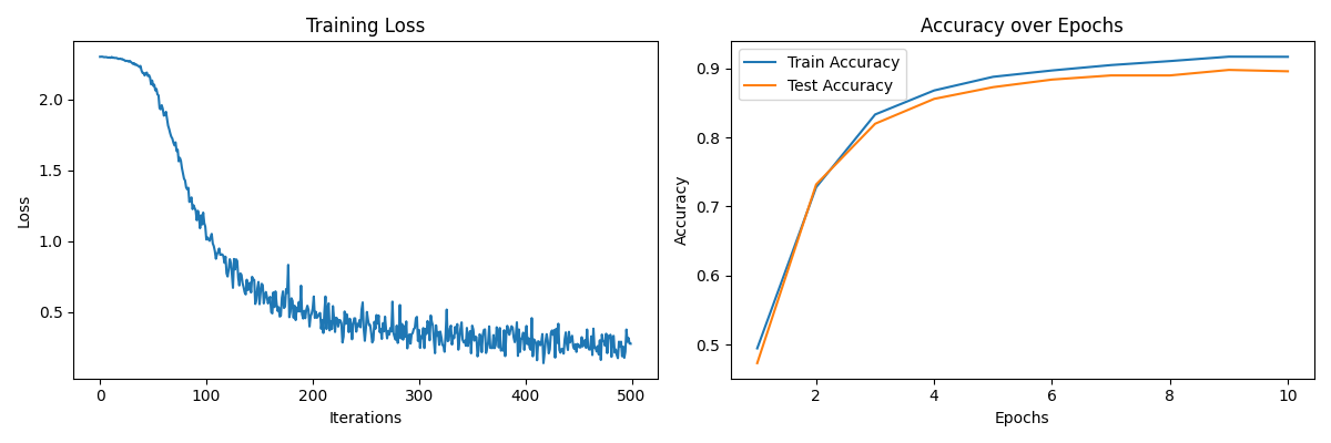
更多推荐
 7
7 0
0- 0


 已为社区贡献1条内容

所有评论(0)