
快速上手大模型:机器学习4(特征缩放、学习率选择、特征工程、多项式回归)
·
目录
1.2.2 均值归一化(Mean normalization)
1.2.3 Z-score归一化(Z-score normalization)
5 多项式回归(Polynomial Regression)
1 特征缩放
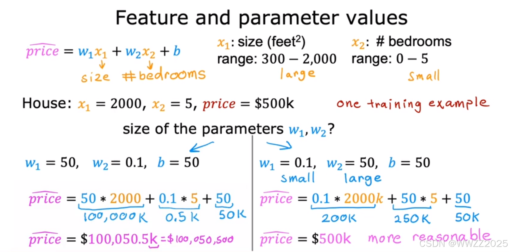
1.1 引子
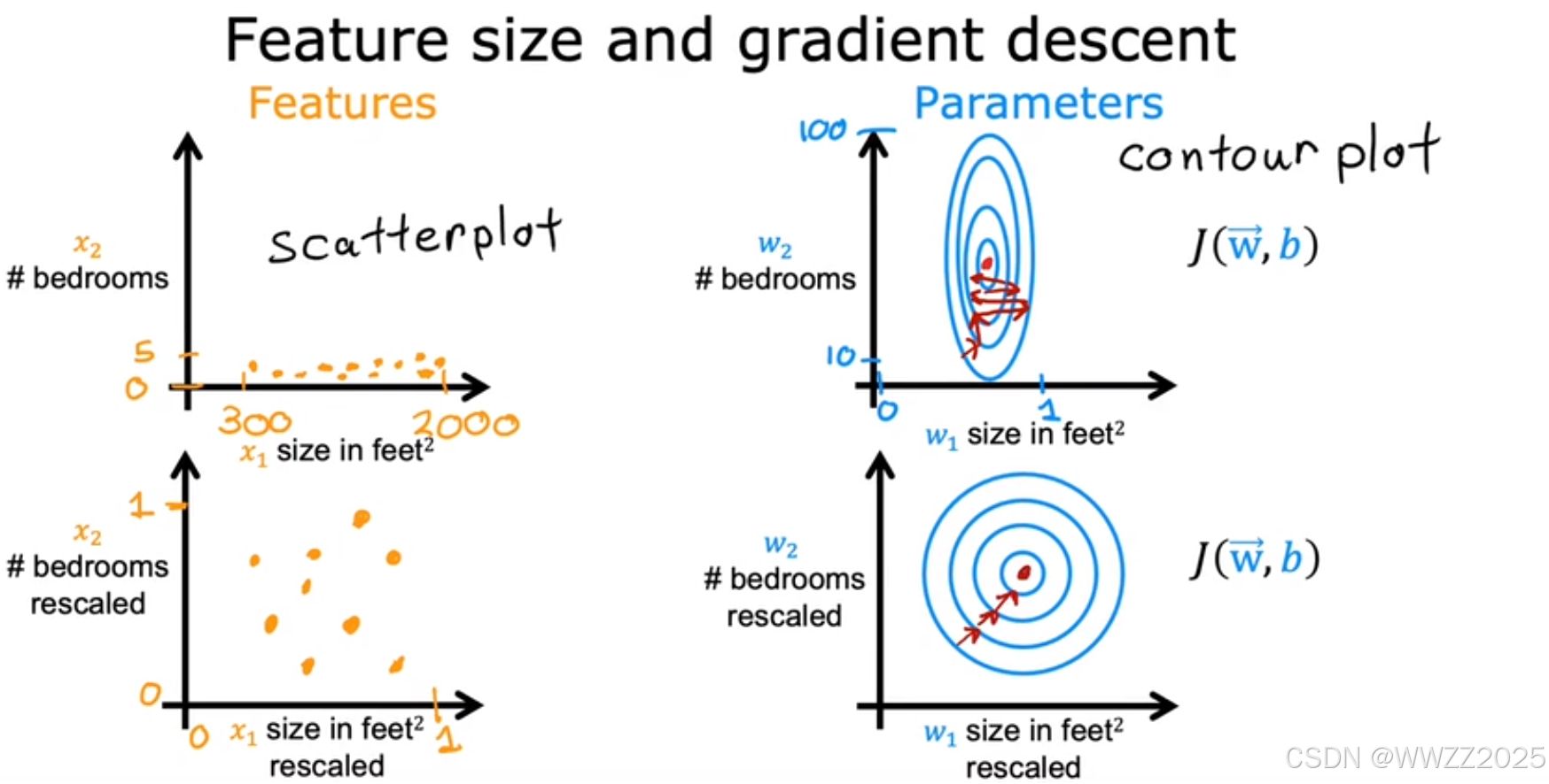
结论:通过缩放w1*x1、w2*x2使其数值差接近,使用转换后的数据运行梯度下降算法,等高线类似于圆,梯度下降可以找到一条更直接的路径到达全局最小值。
1.2 缩放方法
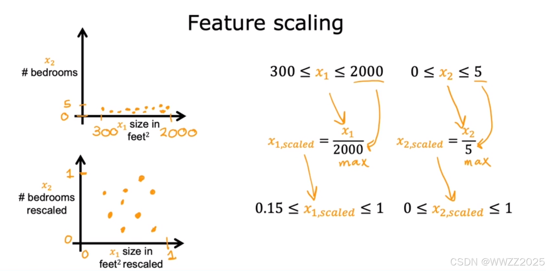
1.2.1 除以最大值法
除以区间最大值,使缩放后的点落在一个近圆上。
1.2.2 均值归一化(Mean normalization)
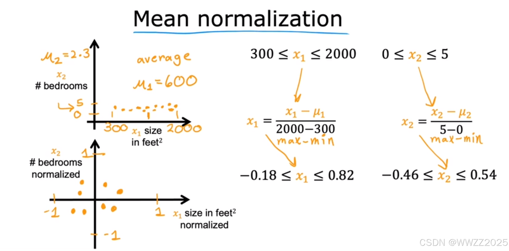
缩放后使x1、x2在-1~1之间分布。
、
分别是x1、x2在训练集上的均值,然后用每个x1、x2算放缩后的值,找出放缩后的范围。
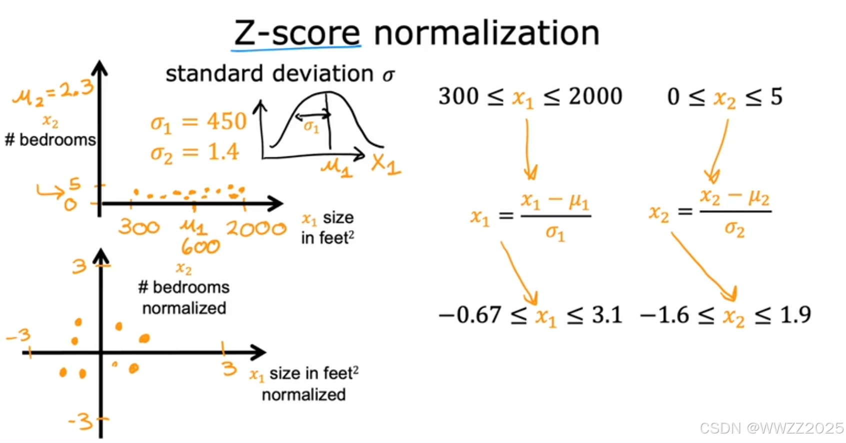
1.2.3 Z-score归一化(Z-score normalization)
归一化公式:
,
其中,
分别是x1、x2在训练集上的均值;
是标准差(
)
2 梯度下降收敛判断
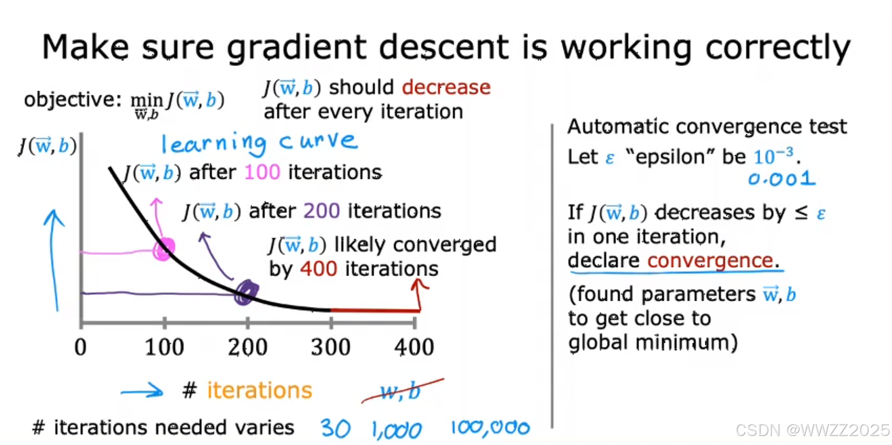
法1:
观察左侧曲线图,迭代至一定次数后基本不再下降,此时即认为收敛。
法2:
自动收敛测试,当J<
时认为收敛,
3 学习率选择(步长)
3.1 理论
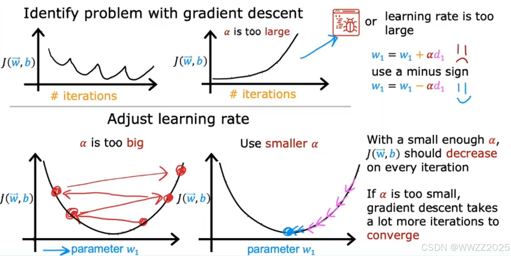
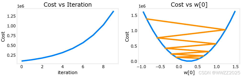
结论:学习率不宜过大或过小,过大出现发散,过小则需要通过更多的迭代次数才能达到收敛。
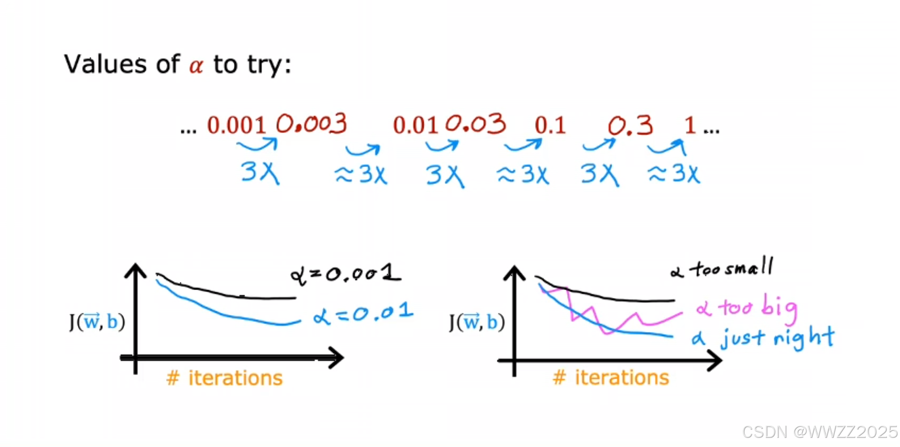
学习率选择:
从0.001开始,0.01、0.1、1进行选择,十倍频程,直至找到蓝色曲线。
3.2 代码实现
3.2.1 代价函数及参数运算
#set alpha to 9.9e-7
_, _, hist = run_gradient_descent(X_train, y_train, 10, alpha = 9.9e-7)
输出:
Iteration Cost          w0       w1       w2       w3       b       djdw0    djdw1    djdw2    djdw3    djdb
---------------------|--------|--------|--------|--------|--------|--------|--------|--------|--------|--------|
        0 9.55884e+04  5.5e-01  1.0e-03  5.1e-04  1.2e-02  3.6e-04 -5.5e+05 -1.0e+03 -5.2e+02 -1.2e+04 -3.6e+02
        1 1.28213e+05 -8.8e-02 -1.7e-04 -1.0e-04 -3.4e-03 -4.8e-05  6.4e+05  1.2e+03  6.2e+02  1.6e+04  4.1e+02
        2 1.72159e+05  6.5e-01  1.2e-03  5.9e-04  1.3e-02  4.3e-04 -7.4e+05 -1.4e+03 -7.0e+02 -1.7e+04 -4.9e+02
        3 2.31358e+05 -2.1e-01 -4.0e-04 -2.3e-04 -7.5e-03 -1.2e-04  8.6e+05  1.6e+03  8.3e+02  2.1e+04  5.6e+02
        4 3.11100e+05  7.9e-01  1.4e-03  7.1e-04  1.5e-02  5.3e-04 -1.0e+06 -1.8e+03 -9.5e+02 -2.3e+04 -6.6e+02
        5 4.18517e+05 -3.7e-01 -7.1e-04 -4.0e-04 -1.3e-02 -2.1e-04  1.2e+06  2.1e+03  1.1e+03  2.8e+04  7.5e+02
        6 5.63212e+05  9.7e-01  1.7e-03  8.7e-04  1.8e-02  6.6e-04 -1.3e+06 -2.5e+03 -1.3e+03 -3.1e+04 -8.8e+02
        7 7.58122e+05 -5.8e-01 -1.1e-03 -6.2e-04 -1.9e-02 -3.4e-04  1.6e+06  2.9e+03  1.5e+03  3.8e+04  1.0e+03
        8 1.02068e+06  1.2e+00  2.2e-03  1.1e-03  2.3e-02  8.3e-04 -1.8e+06 -3.3e+03 -1.7e+03 -4.2e+04 -1.2e+03
        9 1.37435e+06 -8.7e-01 -1.7e-03 -9.1e-04 -2.7e-02 -5.2e-04  2.1e+06  3.9e+03  2.0e+03  5.1e+04  1.4e+03
w,b found by gradient descent: w: [-0.87 -0.   -0.   -0.03], b: -0.00
3.2.2 图像绘制
plot_cost_i_w(X_train, y_train, hist)输出:
3.2.3 Z-score归一化
def zscore_normalize_features(X):
    """
    computes  X, zcore normalized by column

    Args:
      X (ndarray): Shape (m,n) input data, m examples, n features

    Returns:
      X_norm (ndarray): Shape (m,n)  input normalized by column
      mu (ndarray):     Shape (n,)   mean of each feature
      sigma (ndarray):  Shape (n,)   standard deviation of each feature
    """
    # find the mean of each column/feature
    mu     = np.mean(X, axis=0)                 # mu will have shape (n,)
    # find the standard deviation of each column/feature
    sigma  = np.std(X, axis=0)                  # sigma will have shape (n,)
    # element-wise, subtract mu for that column from each example, divide by std for that column
    X_norm = (X - mu) / sigma

    return (X_norm, mu, sigma)

#check our work
#from sklearn.preprocessing import scale
#scale(X_orig, axis=0, with_mean=True, with_std=True, copy=True)

mu     = np.mean(X_train,axis=0)
sigma  = np.std(X_train,axis=0)
X_mean = (X_train - mu)
X_norm = (X_train - mu)/sigma

fig,ax=plt.subplots(1, 3, figsize=(12, 3))
ax[0].scatter(X_train[:,0], X_train[:,3])
ax[0].set_xlabel(X_features[0]); ax[0].set_ylabel(X_features[3]);
ax[0].set_title("unnormalized")
ax[0].axis('equal')

ax[1].scatter(X_mean[:,0], X_mean[:,3])
ax[1].set_xlabel(X_features[0]); ax[0].set_ylabel(X_features[3]);
ax[1].set_title(r"X - $\mu$")
ax[1].axis('equal')

ax[2].scatter(X_norm[:,0], X_norm[:,3])
ax[2].set_xlabel(X_features[0]); ax[0].set_ylabel(X_features[3]);
ax[2].set_title(r"Z-score normalized")
ax[2].axis('equal')
plt.tight_layout(rect=[0, 0.03, 1, 0.95])
fig.suptitle("distribution of features before, during, after normalization")
plt.show()
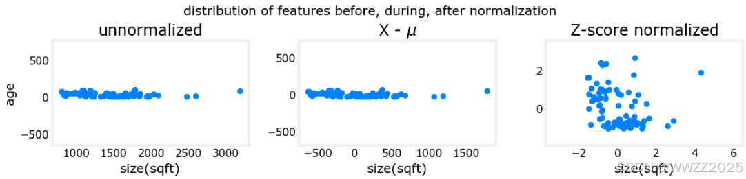
输出:
4 特征工程
4.1 引子
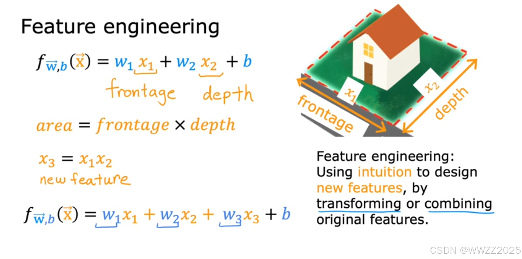
接房价预测示例,x1为房屋所在土地宽度(frontage)、x2为地块深度(depth),如此可以建立模型
;
又因面积=x1*x2;
另x3=x1*x2,新特征x3即为土地面积。
4.2 定义
通过转化、组合问题的原始特征,以便让学习算法更容易作出准确预测。
5 多项式回归(Polynomial Regression)
5.1 引子
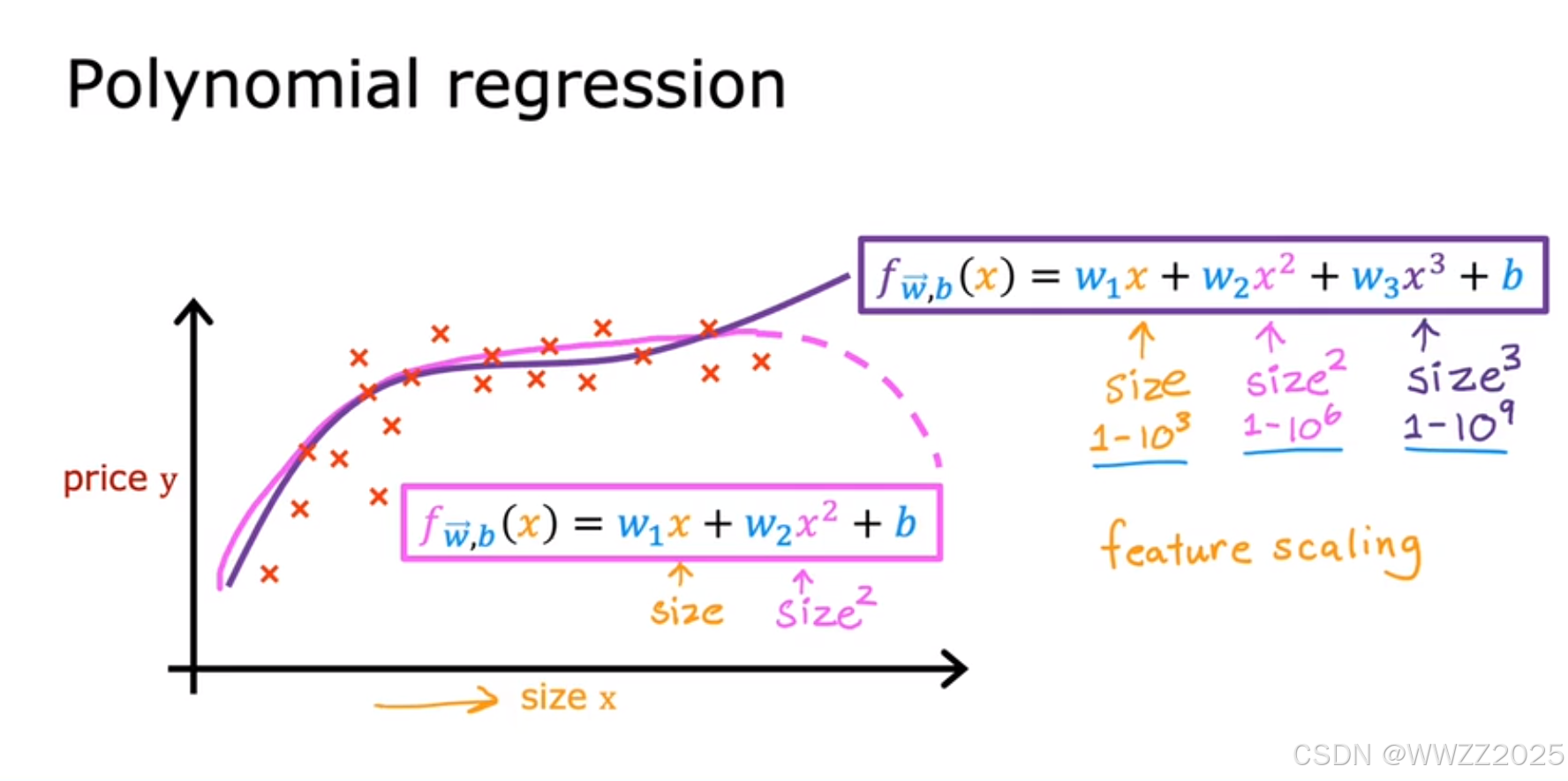
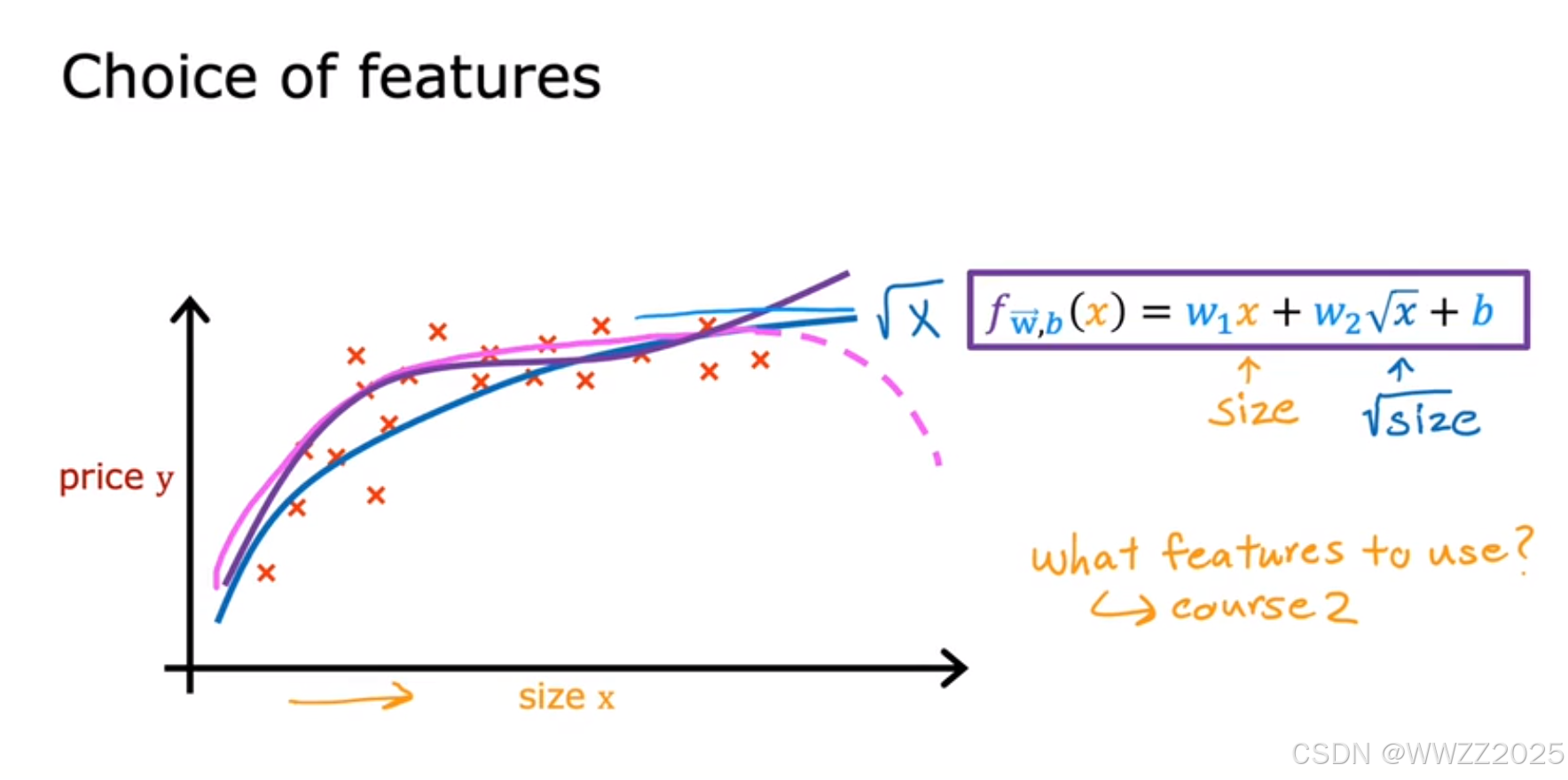
根据实际场景,选择合理的模型。
理论上房子面积越大,房价越贵,故可以选择这两种模型:
5.2 代码示例
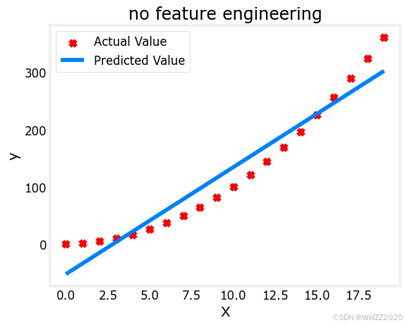
拟合非线性曲线,当模型为y=wx+b时,实际曲线(红色)与预测曲线(蓝色)存在较大出入。
# create target data
x = np.arange(0, 20, 1)
y = 1 + x**2
X = x.reshape(-1, 1)

model_w,model_b = run_gradient_descent_feng(X,y,iterations=1000, alpha = 1e-2)

plt.scatter(x, y, marker='x', c='r', label="Actual Value"); plt.title("no feature engineering")
plt.plot(x,X@model_w + model_b, label="Predicted Value");  plt.xlabel("X"); plt.ylabel("y"); plt.legend(); plt.show()
输出:
Iteration         0, Cost: 1.65756e+03
Iteration       100, Cost: 6.94549e+02
Iteration       200, Cost: 5.88475e+02
Iteration       300, Cost: 5.26414e+02
Iteration       400, Cost: 4.90103e+02
Iteration       500, Cost: 4.68858e+02
Iteration       600, Cost: 4.56428e+02
Iteration       700, Cost: 4.49155e+02
Iteration       800, Cost: 4.44900e+02
Iteration       900, Cost: 4.42411e+02
w,b found by gradient descent: w: [18.7], b: -52.0834
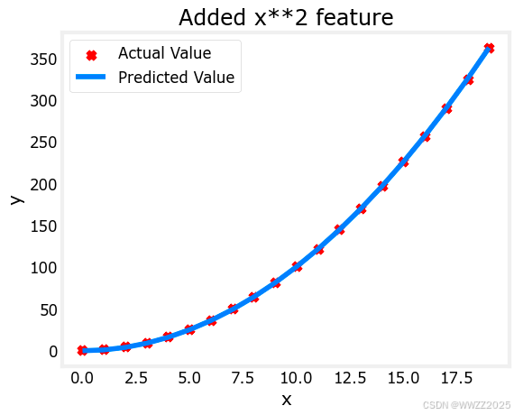
当使用特征工程的思想,将模型变为y=wx^2+b,图像近似重合。
# create target data
x = np.arange(0, 20, 1)
y = 1 + x**2

# Engineer features
X = x**2      #<-- added engineered feature

X = X.reshape(-1, 1)  #X should be a 2-D Matrix
model_w,model_b = run_gradient_descent_feng(X, y, iterations=10000, alpha = 1e-5)

plt.scatter(x, y, marker='x', c='r', label="Actual Value"); plt.title("Added x**2 feature")
plt.plot(x, np.dot(X,model_w) + model_b, label="Predicted Value"); plt.xlabel("x"); plt.ylabel("y"); plt.legend(); plt.show()
输出:
Iteration         0, Cost: 7.32922e+03
Iteration      1000, Cost: 2.24844e-01
Iteration      2000, Cost: 2.22795e-01
Iteration      3000, Cost: 2.20764e-01
Iteration      4000, Cost: 2.18752e-01
Iteration      5000, Cost: 2.16758e-01
Iteration      6000, Cost: 2.14782e-01
Iteration      7000, Cost: 2.12824e-01
Iteration      8000, Cost: 2.10884e-01
Iteration      9000, Cost: 2.08962e-01
w,b found by gradient descent: w: [1.], b: 0.0490
5.3 通用调参示例
5.3.1 不使用归一化
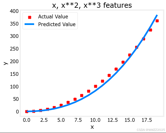
模型使用y=w1x+w2x^2+w3x^3+b
# create target data
x = np.arange(0, 20, 1)
y = x**2

# engineer features .
X = np.c_[x, x**2, x**3]   #<-- added engineered feature

model_w,model_b = run_gradient_descent_feng(X, y, iterations=10000, alpha=1e-7)

plt.scatter(x, y, marker='x', c='r', label="Actual Value"); plt.title("x, x**2, x**3 features")
plt.plot(x, X@model_w + model_b, label="Predicted Value"); plt.xlabel("x"); plt.ylabel("y"); plt.legend(); plt.show()
输出:
Iteration         0, Cost: 1.14029e+03
Iteration      1000, Cost: 3.28539e+02
Iteration      2000, Cost: 2.80443e+02
Iteration      3000, Cost: 2.39389e+02
Iteration      4000, Cost: 2.04344e+02
Iteration      5000, Cost: 1.74430e+02
Iteration      6000, Cost: 1.48896e+02
Iteration      7000, Cost: 1.27100e+02
Iteration      8000, Cost: 1.08495e+02
Iteration      9000, Cost: 9.26132e+01
w,b found by gradient descent: w: [0.08 0.54 0.03], b: 0.0106
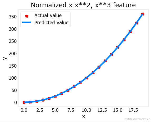
5.3.2 使用Z-score归一化
# create target data
x = np.arange(0,20,1)
X = np.c_[x, x**2, x**3]
print(f"Peak to Peak range by column in Raw        X:{np.ptp(X,axis=0)}")

# add mean_normalization
X = zscore_normalize_features(X)
print(f"Peak to Peak range by column in Normalized X:{np.ptp(X,axis=0)}")

x = np.arange(0,20,1)
y = x**2

X = np.c_[x, x**2, x**3]
X = zscore_normalize_features(X)

model_w, model_b = run_gradient_descent_feng(X, y, iterations=100000, alpha=1e-1)

plt.scatter(x, y, marker='x', c='r', label="Actual Value"); plt.title("Normalized x x**2, x**3 feature")
plt.plot(x,X@model_w + model_b, label="Predicted Value"); plt.xlabel("x"); plt.ylabel("y"); plt.legend(); plt.show()
输出:
Iteration         0, Cost: 9.42147e+03
Iteration     10000, Cost: 3.90938e-01
Iteration     20000, Cost: 2.78389e-02
Iteration     30000, Cost: 1.98242e-03
Iteration     40000, Cost: 1.41169e-04
Iteration     50000, Cost: 1.00527e-05
Iteration     60000, Cost: 7.15855e-07
Iteration     70000, Cost: 5.09763e-08
Iteration     80000, Cost: 3.63004e-09
Iteration     90000, Cost: 2.58497e-10
w,b found by gradient descent: w: [5.27e-05 1.13e+02 8.43e-05], b: 123.5000
结论:近似拟合
更多推荐

 9
9 0
0- 0


 已为社区贡献23条内容

所有评论(0)