目标读者：无编程与无机器学习实战基础，希望能用 Julia 独立完成鸢尾花（Iris）数据集的逻辑回归分类，并逐步达到能优化和部署模型的水平。
结构：基础 → 生态 → 理论 + 手动实现 → 实战整合 → 进阶优化 → 资源与故障排查。每个知识点含理论讲解 + 代码示例 + 注释说明，按步骤编号，代码可直接复制运行。

---

一、教程定位

1. 受众：Julia 零基础 + 机器学习实战经验为零。
2. 深度：从基础语法、包管理、数值运算，到 ML 生态、手写逻辑回归、调用库实现、评估、优化、部署。
3. 形式：每一模块按顺序展开；每步都有可运行代码或明确命令；重点用粗体标注。

---

二、核心内容模块

模块1：Julia 入门必备（安装与语法基础）

1.1 环境搭建（Windows / macOS / Linux）

目标：能运行 Julia REPL、在编辑器中编写与运行脚本、在 Notebook 中迭代开发。

1. 安装 Julia：

   • 访问官方下载安装包（选择与你系统匹配的 stable 版）。

   • Julia官网：https://julialang.org/

   • Julia 中文手册：https://docs.juliacn.com/latest/

     • Windows：下载 .exe 安装或 .zip；macOS：.dmg；Linux：.tar.gz 解压并把 bin 加入 PATH。

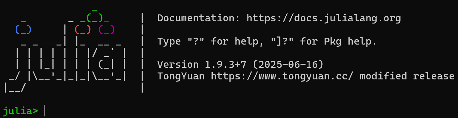
   • 验证：终端执行 julia，应进入 REPL（类似命令行界面）。
     

2. 推荐 IDE / 编辑器：

   • VS Code + Julia 扩展（强烈推荐）：安装 VS Code → 扩展市场搜索 “Julia” 并安装。支持调试、自动补全、Plot 显示、REPL 集成。
     * Jupyter Notebook / JupyterLab（IJulia）：在 Julia REPL 运行 using Pkg; Pkg.add("IJulia")，然后在终端 jupyter lab 启动。
   • 轻量：直接在 REPL 或 Atom + Juno（可选）。

3. 在 VS Code 中配置：

   • 安装 Julia 扩展后，在设置里指定 julia.executablePath 为 Julia 可执行路径（例如 C:\Program Files\Julia\Julia-1.x\bin\julia.exe）。
   • 推荐安装 JuliaFormatter、LanguageServer.jl（自动在扩展中提示安装）。

1.2 包管理（Pkg）

目标：会创建环境、安装与管理包。

# 打开 Julia REPL，按 ] 进入 Pkg 模式：
] activate MyIrisEnv       # 创建并激活项目环境
] add DataFrames CSV Plots StatsBase LinearAlgebra MLJ RDatasets GLM Optim Flux ScikitLearn JLD2
] instantiate              # 可选：安装已记录依赖

• activate：为项目创建隔离环境（类似 Python 的 venv）。
• 在脚本中使用：

using Pkg
Pkg.activate("MyIrisEnv")   # 在脚本里也可激活

1.3 核心基础语法（变量、类型、流程控制、函数）

目标：掌握 Julia 基本语法（和其他语言的差异）。示例极简说明常用语法。

# 变量与类型
x = 3.14        # 自动类型推断 Float64
y::Int = 2      # 指定类型

# 基本运算
z = x + y
arr = [1, 2, 3]         # 一维数组（Vector）
mat = [1 2; 3 4]        # 矩阵

# 流程控制
for i in 1:5
    println(i)
end

if x > 1
    println("x>1")
else
    println("x<=1")
end

# 函数定义
function sigmoid(z)
    1 ./ (1 .+ exp.(-z))   # element-wise 运算
end

# 匿名函数
f = x -> x^2

# 多重返回值
function divmod(a,b)
    return div(a,b), rem(a,b)
end

注：Julia 使用 . 运算符做元素级广播（exp.、.+、./），这是 Julia 的重要习惯用法，便于向量化运算。

1.4 数据结构（数组、矩阵、字典、元组）

1. 数组（Vector）：一维可变长度容器。
2. 矩阵（Matrix）：2D 数组，常用于数值计算与线性代数。
3. 字典（Dict）：键值对。
4. 元组（Tuple）：不可变序列（轻量）。

示例：

v = Int[1,2,3]
m = Float64[1 2 3; 4 5 6]
d = Dict("a"=>1, "b"=>2)
t = (1, "two", 3.0)

适配 ML 场景：DataFrames（见下）更适合表格数据处理；矩阵常用于数值线性代数计算（训练模型时的 X、y）。

1.5 与其他语言的语法差异（快速对比）

• 索引从 1 开始（非 0）：arr[1] 是第一个元素。
• 广播（.）语法：元素级运算用 .（比 Python 更显式且高效）。
• 类型推断 + JIT 编译：首次运行函数会花时间编译，但后续很快。
• 多重返回、强大的元编程（macro），但初学者先不必深入。

---

模块2：Julia 机器学习生态铺垫

2.1 常用 ML 相关库（简介与适用场景）

1. DataFrames.jl：表格数据处理，类似 pandas。主要用于数据清洗与探索。
2. CSV.jl：读取/写入 CSV 文件。
3. RDatasets.jl：快速获得经典数据集（如 iris）。
4. StatsBase.jl：基础统计/评估工具（混淆矩阵、采样等）。
5. Plots.jl / Makie.jl：绘图（Plots 适合入门）。
6. GLM.jl：统计建模（一般线性/广义线性模型），可用于二分类逻辑回归（包良好）。
7. MLJ.jl：Julia 的机器学习框架，类似 scikit-learn 的统一接口，便于做模型比较与调参。
8. Flux.jl：深度学习框架（神经网络），若要做更复杂模型用它。
9. ScikitLearn.jl：包装 Python scikit-learn（便于熟悉 scikit-learn 的用户）。
10. JLD2.jl：模型/数据持久化（保存与加载）。

2.2 数据处理基础（鸢尾花示例）

步骤

1. 使用 RDatasets 加载 Iris：

using RDatasets, DataFrames
iris = dataset("datasets", "iris")   # DataFrame 格式
first(iris, 5)

2. 查看摘要：

describe(iris)

3. 可视化（用 Plots）：

using Plots, StatsPlots
@df iris scatter(:SepalLength, :SepalWidth, group=:Species, title="Sepal Length vs Width")

注：@df 宏来自 StatsPlots，使 DataFrame 绘图更方便。

2.3 数值计算基础（矩阵运算、线性代数）

• 使用 LinearAlgebra：矩阵乘法 *、点乘 .、转置 transpose 或 '。
• 常见操作：

using LinearAlgebra
X = rand(150,4)  # 150x4 矩阵
theta = rand(4)
y_pred = X * theta  # 线性组合

重要：向量化实现会比逐元素循环快很多；Julia 在向量化与广播上都很高效。

---

模块3：机器学习基础与逻辑回归详解

3.1 逻辑回归核心理论（简洁）

1. 目标：输入特征 → 预测二分类或多分类概率。
2. 二分类：使用 sigmoid 函数把线性模型输出转为概率：
   $$\hat{p}=\sigma (X\theta )=\frac{1}{1+e^{-X\theta }}$$
   其中，$\hat{p}$ 为预测概率，$X$ 为特征矩阵，$\theta$ 为参数向量，$\sigma$ 为Sigmoid激活函数。
3. 损失函数：对数损失（Binary cross-entropy）：
   $$J(\theta )=-\frac{1}{m}\sum _{i=1}^m\left[y^{(i)}\log {\hat{p}}^{(i)}+(1-y^{(i)})\log (1-{\hat{p}}^{(i)})\right]$$
4. 优化：梯度下降（batch / mini-batch / 使用优化库如 Optim.jl 或 GLM.jl 的拟合器）。
5. 多分类（softmax / one-vs-rest）：Softmax 多项逻辑回归或将 K 类转为 K 个二分类 (One-vs-Rest)。

3.2 手动实现逻辑回归（从底层到多分类）

下面给出从**标准化输入 → 手写 Softmax 多分类逻辑回归（批量梯度下降）**的完整代码。该实现便于学习内部细节。

代码：手写多类逻辑回归（Softmax）

# 手写 Softmax 逻辑回归（鸢尾花，多类）
using RDatasets, DataFrames, Random, LinearAlgebra, Statistics, StatsBase

# 1. 加载数据
iris = dataset("datasets", "iris")
# 取特征和标签
X = Matrix(iris[:, 1:4])  # 150 x 4
labels = iris[:, :Species] # CategoricalValue

# 2. 将 label 转为整数 1,2,3
label_map = Dict(level => i for (i, level) in enumerate(levels(labels)))
y = [label_map[l] for l in labels]  # 1..3

# 3. 标准化特征（零均值，单位方差）
X_mean = mean(X, dims=1)
X_std = std(X, dims=1, corrected=true)
X_std[X_std .== 0] .= 1.0  # 防止除0
X_norm = (X .- X_mean) ./ X_std

# 4. 添加偏置列
m, n = size(X_norm)
Xb = hcat(ones(m), X_norm)  # m x (n+1)

# 5. one-hot 编码标签
K = length(unique(y))
Y_onehot = zeros(m, K)
for i in 1:m
    Y_onehot[i, y[i]] = 1.0
end

# 6. 初始化参数
Random.seed!(123)
Θ = 0.01 * randn(n+1, K)  # (n+1) x K

# 7. softmax 函数
function softmax(Z)
    # Z: m x K
    Zmax = maximum(Z, dims=2)
    expZ = exp.(Z .- Zmax)         # 稳定性：减去行最大值
    expZ ./ sum(expZ, dims=2)
end

# 8. 交叉熵损失
function cross_entropy(Y_hat, Y)
    -mean(sum(Y .* log.(Y_hat .+ 1e-12), dims=2))
end

# 9. 训练（批量梯度下降）
function train!(Θ, Xb, Y_onehot; lr=0.1, epochs=1000)
    m = size(Xb, 1)
    for epoch in 1:epochs
        Z = Xb * Θ                    # m x K
        Y_hat = softmax(Z)            # m x K
        loss = cross_entropy(Y_hat, Y_onehot)
        # gradient : (n+1) x K
        grad = (Xb' * (Y_hat .- Y_onehot)) ./ m
        Θ .-= lr .* grad
        if epoch % 100 == 0
            println("epoch=$epoch, loss=$(round(loss, digits=6))")
        end
    end
end

# 10. 预测函数
function predict(Θ, Xb)
    P = softmax(Xb * Θ)  # m x K
    return map(i -> argmax(P[i, :]), 1:size(P,1))
end

# 11. 训练模型
train!(Θ, Xb, Y_onehot, lr=0.5, epochs=1000)

# 12. 评估
y_pred = collect(predict(Θ, Xb))
accuracy = mean(y_pred .== y)
println("训练集准确率: ", round(accuracy*100, digits=2), "%")

注释说明：

• 数据标准化 是训练逻辑回归重要步骤（加快收敛，避免某个特征占主导）。
• softmax 实现 使用数值稳定性技巧（减去每行最大值）。
• 梯度 计算：(X^T * (Y_hat - Y)) / m。
• 该实现使用 batch 梯度下降；可扩展为 mini-batch 或使用优化库。

3.3 使用 ML 库快速实现（对比）

方案一：GLM.jl（广义线性模型） —— 适合二分类（使用 Bernoulli 家族），对于多分类需做 one-vs-rest 或用其它包。

using DataFrames, GLM, RDatasets, StatsModels

iris = dataset("datasets", "iris")
# 将 Species 转为二分类示例（只取 setosa 与 versicolor）
df2 = filter(row -> row.Species != "virginica", iris)
df2.Species = categorical(df2.Species)

# 拟合二分类逻辑回归
m = glm(@formula(Species ~ SepalLength + SepalWidth + PetalLength + PetalWidth),
        df2, Binomial(), LogitLink())

coeftable(m)

方案二：ScikitLearn.jl（包装 scikit-learn）或 MLJ.jl —— 方便训练多分类模型并直接获得交叉验证与调参工具。示例（ScikitLearn）：

using ScikitLearn, ScikitLearn.CrossValidation: train_test_split
@sk_import linear_model: LogisticRegression
@sk_import preprocessing: StandardScaler
using RDatasets, DataFrames

iris = dataset("datasets", "iris")
X = Matrix(iris[:,1:4])
y = iris[:, :Species] |> x -> collect(levelcode.(categorical(x)))  # 数字标签

# 标准化 + 划分
scaler = StandardScaler()
Xs = fit_transform!(scaler, X)
X_train, X_test, y_train, y_test = train_test_split(Xs, y, test_size=0.2, random_state=42)

clf = LogisticRegression(multi_class="multinomial", solver="lbfgs", max_iter=200)
fit!(clf, X_train, y_train)
println("准确率（测试集）：", score(clf, X_test, y_test))

对比：

• 手工实现：完全控制、学习内部机制，但效率/稳定性/功能有限。
• 库实现（GLM/MLJ/ScikitLearn）：功能全面（正则、优化器、评估、CV），适合生产或快速实验。

3.4 模型评估指标（代码实现）

关键指标：准确率（accuracy）、精确率（precision）、召回率（recall）、F1、混淆矩阵。

示例（基于 StatsBase）：

using StatsBase

# y_true: [1..K], y_pred: [1..K]
function confusion_matrix(y_true, y_pred; labels=unique(y_true))
    cm = zeros(Int, length(labels), length(labels))
    label_index = Dict(l => i for (i,l) in enumerate(labels))
    for (yt, yp) in zip(y_true, y_pred)
        cm[label_index[yt], label_index[yp]] += 1
    end
    return cm
end

cm = confusion_matrix(y, y_pred, labels=[1,2,3])
println("混淆矩阵：")
println(cm)

# 精确率/召回率（按类别）
function precision_recall_f1(cm)
    TP = diag(cm)
    FP = sum(cm, dims=1)' .- TP
    FN = sum(cm, dims=2) .- TP
    precision = TP ./ (TP .+ FP)
    recall = TP ./ (TP .+ FN)
    f1 = 2 .* (precision .* recall) ./ (precision .+ recall)
    return precision, recall, f1
end

precision, recall, f1 = precision_recall_f1(cm)
println("Precision:", precision, " Recall:", recall, " F1:", f1)

---

模块4：实战项目 —— 鸢尾花分类完整流程

目标：从载入数据、预处理、模型（手写 + 库）训练到评估与可视化，提交一个能直接运行的整套代码。

4.1 完整流程概览（步骤编号）

1. 准备环境与安装包（见模块1）。
2. 加载数据（RDatasets 或 CSV）。
3. EDA（基本统计、可视化）。
4. 预处理（编码、标准化、训练/测试划分）。
5. 模型一：手动实现 Softmax 逻辑回归（参考模块3）。
6. 模型二：使用 ScikitLearn.jl 或 MLJ.jl 训练多项逻辑回归。
7. 超参数调优（学习率、正则化），交叉验证。
8. 评估与可视化（混淆矩阵、ROC（多类需多对一）、分类报告）。
9. 保存模型并展示如何加载与预测新样本。

4.2 完整代码（整合，可直接运行）

把前面组件整合成一个脚本 iris_logistic.jl（注：确保已在环境中 add 需要的包）。

# iris_logistic.jl -- 完整示例
using Pkg
# Pkg.activate("MyIrisEnv")  # 可选：在项目环境运行
using RDatasets, DataFrames, Random, LinearAlgebra, Statistics, StatsBase, Plots
# 1. 加载数据
iris = dataset("datasets", "iris")
first(iris,5)

# 2. 特征和标签
X = Matrix(iris[:, 1:4])
labels = iris[:, :Species]
label_map = Dict(level => i for (i, level) in enumerate(levels(labels)))
y = [label_map[l] for l in labels]

# 3. 标准化
X_mean = mean(X, dims=1)
X_std = std(X, dims=1, corrected=true)
X_norm = (X .- X_mean) ./ X_std
Xb = hcat(ones(size(X,1)), X_norm)  # 添加偏置

# 4. 划分训练/测试（80/20）
Random.seed!(42)
indices = collect(1:size(Xb,1))
shuffle!(indices)
train_idx = indices[1:120]
test_idx = indices[121:end]

X_train = Xb[train_idx, :]
X_test = Xb[test_idx, :]
y_train = y[train_idx]
y_test = y[test_idx]

# 5. one-hot 训练标签
K = length(unique(y))
Y_train = zeros(length(train_idx), K)
for (i, lab) in enumerate(y_train)
    Y_train[i, lab] = 1.0
end

# 6. 初始化 Theta
Θ = 0.01 * randn(size(X_train,2), K)

# 7. softmax / loss / grad
function softmax(Z)
    Zm = maximum(Z, dims=2)
    exp.(Z .- Zm) ./ sum(exp.(Z .- Zm), dims=2)
end

function cross_entropy(Y_hat, Y)
    -mean(sum(Y .* log.(Y_hat .+ 1e-12), dims=2))
end

# 8. 训练函数（带正则）
function train!(Θ, X, Y; lr=0.5, epochs=1000, λ=0.0)
    m = size(X,1)
    for epoch in 1:epochs
        Z = X * Θ
        Y_hat = softmax(Z)
        loss = cross_entropy(Y_hat, Y) + (λ/(2m)) * sum(Θ[2:end,:].^2)  # L2 正则（不正则偏置）
        grad = (X' * (Y_hat .- Y)) ./ m
        grad[2:end, :] .+= (λ/m) .* Θ[2:end, :]  # 正则项不包含偏置
        Θ .-= lr .* grad
        if epoch % 200 == 0
            println("epoch=$epoch loss=$(round(loss,digits=6))")
        end
    end
end

# 9. 训练
train!(Θ, X_train, Y_train, lr=0.5, epochs=1000, λ=0.01)

# 10. 预测函数
function predict_labels(Θ, X)
    P = softmax(X * Θ)
    return [argmax(P[i,:]) for i in 1:size(P,1)]
end

y_pred_train = predict_labels(Θ, X_train)
y_pred_test = predict_labels(Θ, X_test)

# 11. 评估
function report(y_true, y_pred)
    acc = mean(y_true .== y_pred)
    cm = zeros(Int, K, K)
    for (t,p) in zip(y_true, y_pred)
        cm[t,p] += 1
    end
    precision, recall, f1 = precision_recall_f1(cm)
    return acc, cm, precision, recall, f1
end

acc_train, cm_train, pr_train, rc_train, f1_train = report(y_train, y_pred_train)
acc_test, cm_test, pr_test, rc_test, f1_test = report(y_test, y_pred_test)

println("Train acc: ", round(acc_train*100, digits=2), "%")
println("Test acc: ", round(acc_test*100, digits=2), "%")
println("Test Confusion Matrix:\n", cm_test)
println("Test Precision: ", round.(pr_test, digits=3))
println("Test Recall: ", round.(rc_test, digits=3))
println("Test F1: ", round.(f1_test, digits=3))

# 12. 可视化（2D 投影）
# 使用前两维绘图，仅作示意
x_plot = X[test_idx, 2]  # 原始第1特征（标准化后）
y_plot = X[test_idx, 3]  # 原始第2特征（标准化后）
scatter(x_plot, y_plot, group=y_test, markerstrokewidth=0, label="True")
scatter!(x_plot, y_plot, group=y_pred_test, markershape=:xcross, ms=4, label="Pred")

注：

• 该脚本展示了训练/测试划分、正则、评估与可视化；读者可直接在 VS Code 的 Julia REPL 或 Jupyter 中运行。
• 若想使用 GLM/MLJ 替代手写模型，参见模块3 中的示例。

---

模块5：进阶提升

5.1 Julia 性能优化

1. 避免全局变量：把变量放进函数或 let 块，以便编译器类型稳定。

   function run_model(...)
       local_var = ...
   end
   

2. 类型声明：在公共 API 层不必过度声明，但在循环密集处可声明输入类型以避免运行时分派。

3. 向量化与广播：使用 . 广播与矩阵乘法避免显式 for 循环。

4. 多线程/并行：

   • 启动 Julia 时使用 julia -t n 开启 n 线程。
   • 使用 Threads.@threads 并行化 for 循环（需注意数据竞争）。

5. 内存分配与预分配：在循环中避免频繁分配临时数组，采用预先分配的数组并复用。

6. Profile 与 Benchmark：@time, @btime（BenchmarkTools.jl）与 Profile 用于定位瓶颈。

5.2 逻辑回归模型优化

1. 正则化（L1 / L2）：控制过拟合。手写模型中可加入惩罚项（如代码示例的 λ 参数）。
2. 学习率调度：采用下降学习率或自适应优化器（比如使用 Optim.jl 或 LBFGS）。
3. 多项式特征 / 特征交互：用于扩展线性边界，但注意维度爆炸与正则。
4. 特征选择：PCA 或基于模型的重要性选择特征，减少过拟合与计算量。

5.3 其他算法扩展

• 决策树、随机森林：使用 DecisionTree.jl 或通过 MLJ.jl 访问多个实现。
• 迁移逻辑回归思路：理解损失与优化可迁移到 SVM / 神经网路的训练逻辑。

5.4 实际项目部署

1. 模型持久化：使用 JLD2.jl 或 BSON.jl 保存权重与预处理参数：

   using JLD2
   @save "iris_model.jld2" Θ X_mean X_std label_map
   @load "iris_model.jld2" Θ X_mean X_std label_map
   

2. 封装为 API：使用 HTTP.jl 或 Genie.jl 创建 REST 接口，接收 JSON 特征并返回预测结果。简单示例（伪代码）：

   using HTTP, JSON
   function handler(req)
       body = String(req.body)
       feats = JSON.parse(body)["features"]
       # 标准化 -> 预测 -> 返回
       return HTTP.Response(200, JSON.json(result))
   end
   HTTP.serve(handler, "0.0.0.0", 8000)
   

3. Docker 化：把 Julia 运行环境打包进 Docker 容器以便部署（使用官方 Julia 镜像）。

---

模块6：资源推荐与常见问题排查

6.1 官方文档与社区

• Julia 官方文档：语言与标准库指南（强烈推荐常看）。
• DataFrames.jl / MLJ.jl / Flux.jl 文档：各自官方仓库和 README。
• 社区：Julia Discourse，StackOverflow。

6.2 常见错误与解决方案

1. 包安装失败：

   • 问题：网络或 registry 问题。
   • 解决：Pkg.update() / 更换镜像源（国内可配置镜像） / 删除 ~/.julia/registries 并 Pkg.Registry.add 重新添加。

2. 函数运行慢（首次慢）：

   • 原因：JIT 编译（首次调用会编译）。
   • 解决：多次运行或用 PackageCompiler 做预编译（高级）。

3. 类型不匹配 / 性能差：

   • 原因：使用全局变量或混合类型（Any）。
   • 解决：把代码封装进函数、尽可能保持类型稳定。

4. 索引越界 / 下标从 1 开始导致困惑：

   • 提示：Julia 索引从 1 开始，注意与 Python 对比。

5. 绘图在 VS Code/REPL 不显示：

   • 可能需要激活 plot 后端或在 notebook 中运行；可使用 display()。