
11种机器学习模型+SHAP+LIME+多种特征重要性分析+贝叶斯优化超参数+二分类+Stacking+Voting
感谢关注,一起来学习干货。
本期摘要
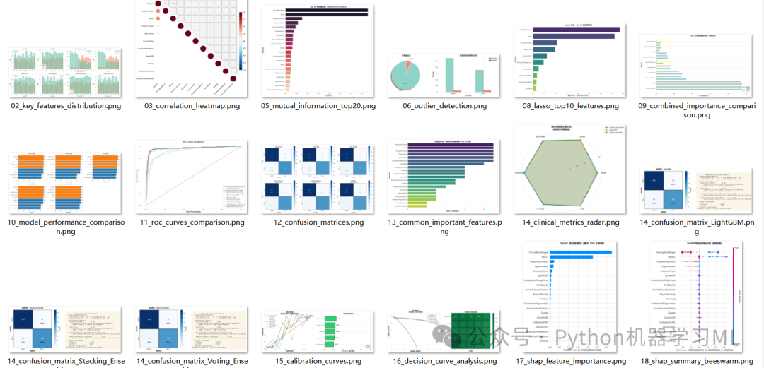
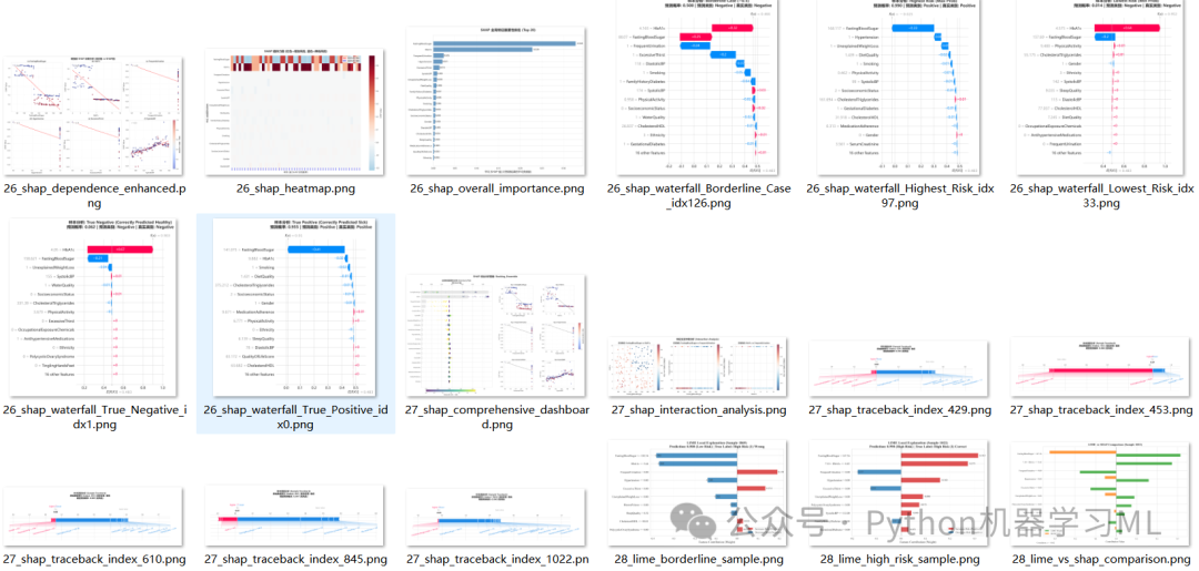
每个阶段都会有详细的介绍和逐行代码注释,确保您能理解每一行代码的作用,并能将其应用到其他数据集中。
阶段 1: 环境设置、数据加载与初步探查
这个阶段负责搭建分析环境,加载数据,并对数据集进行一次快速的“体检”。
作用解释:
- 导入库
导入了
pandas(数据处理)、numpy(数值计算)、matplotlib和seaborn(数据可视化)等核心工具。 - 创建目录
使用
os.makedirs创建了一个专门的输出目录,这是一个良好的编程习惯,能让所有生成的图表和文件有序存放。 - 加载数据
从CSV文件加载数据集。
- 基本信息概览
通过
.shape,.info(),.head()等方法,快速了解数据集的规模(行和列)、每个特征的数据类型、内存占用,并预览数据内容。 - 数据质量检查
使用
.isnull().sum()和.duplicated().sum()检查是否存在缺失值和重复记录,这是数据清洗前最关键的第一步。
# ==================== 导入必要的库 ====================
import numpy as np
import pandas as pd
import matplotlib.pyplot as plt
import seaborn as sns
import warnings
import os
from scipy import stats
from scipy.stats import shapiro, ttest_ind, mannwhitneyu, chi2_contingency
from sklearn.preprocessing import StandardScaler, MinMaxScaler
from sklearn.feature_selection import mutual_info_classif
from sklearn.covariance import EllipticEnvelope
from sklearn.linear_model import lasso_path
from itertools import cycle
import plotly.express as px
import plotly.graph_objects as go
from plotly.subplots import make_subplots

# 忽略警告
warnings.filterwarnings('ignore')

# 设置绘图风格
plt.rcParams['font.sans-serif'] = ['microsoft YaHei']  # 中文字体支持
plt.rcParams['axes.unicode_minus'] = False# 负号显示

# 创建输出目录
output_dir = './diabetes_analysis_results'
os.makedirs(output_dir, exist_ok=True)
print(f"📁 输出目录已创建: {output_dir}")

# ==================== 第一部分:数据加载与基本信息 ====================
print("\n" + "=" * 70)
print("🔍 第一部分:数据基本信息")
print("=" * 70)

# 数据加载
data = pd.read_csv("公众号python机器学习ML-2025-11-28.csv")

print(f"\n📊 数据集形状: {data.shape}")
print(f"📌 特征数量: {data.shape[1] - 1}")
print(f"📌 样本数量: {data.shape[0]}")

print(f"\n📋 数据集信息:")
data.info()

print(f"\n📑 列名列表 ({len(data.columns)} 个):")
for i, col inenumerate(data.columns, 1):
print(f"  {i:2d}. {col}")

print(f"\n👀 前5行数据:")
print(data.head())

print(f"\n🔍 数据质量检查:")
missing_values = data.isnull().sum()
duplicates = data.duplicated().sum()
print(f"  ✓ 缺失值总数: {missing_values.sum()} 个")
print(f"  ✓ 重复记录数: {duplicates} 个")

if missing_values.sum() > 0:
print("\n⚠️ 存在缺失值的列:")
print(missing_values[missing_values > 0])
阶段 2: 探索性数据分析 (EDA)
这个阶段深入分析了目标变量和关键数值特征的分布情况,这是理解数据特性和发现潜在模式的核心步骤。
作用解释:
- 目标变量分析
详细检查了
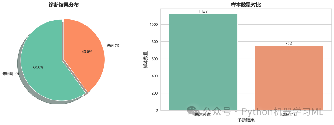
Diagnosis(诊断结果)的分布。结果显示,这是一个类别不平衡的数据集,未患病样本远多于患病样本。这对于后续建模至关重要,因为模型可能会偏向于预测多数类。 - 数值特征统计
使用
.describe()生成了所有数值特征的描述性统计信息(均值、标准差、分位数等),这有助于快速把握每个特征的尺度和分布范围。 - 分布可视化
-
通过饼图和柱状图,直观展示了目标变量的比例和数量。
-
通过直方图(
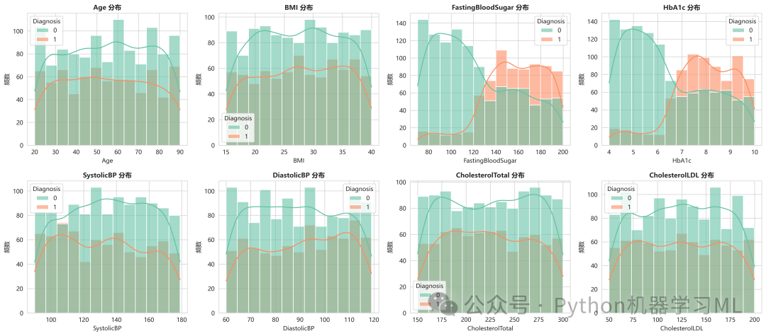
histplot)和核密度估计(kde=True),可视化了几个关键特征(如年龄、BMI、血糖等)的分布。特别地,使用hue='Diagnosis'参数,可以在同一张图上对比患病与未患病群体的特征分布差异,为特征筛选提供直观依据。例如,如果两个群体的分布曲线差异很大,说明该特征区分度高。
-
# ==================== 第二部分:探索性数据分析 ====================
print("\n" + "=" * 70)
print("📊 第二部分:探索性数据分析")
print("=" * 70)

# 目标变量分布
print("\n🎯 目标变量分布分析:")
target_counts = data['Diagnosis'].value_counts()
target_ratio = data['Diagnosis'].value_counts(normalize=True)
print(f"\n类别分布:")
print(f"  未患病 (0): {target_counts[0]} 样本 ({target_ratio[0]*100:.2f}%)")
print(f"  患病   (1): {target_counts[1]} 样本 ({target_ratio[1]*100:.2f}%)")
print(f"  类别比例: 1:{target_counts[0]/target_counts[1]:.2f}")

# 可视化目标变量分布
fig, axes = plt.subplots(1, 2, figsize=(14, 5))
colors_pie = ['#66c2a5', '#fc8d62']

# 饼图
axes[0].pie(
    target_counts,
    labels=['未患病 (0)', '患病 (1)'],
    autopct='%1.1f%%',
    startangle=90,
    colors=colors_pie,
    explode=(0.05, 0),
    shadow=True
)
axes[0].set_title('诊断结果分布', fontsize=14, fontweight='bold')

# 柱状图
sns.countplot(data=data, x='Diagnosis', ax=axes[1], palette=colors_pie)
axes[1].set_title('样本数量对比', fontsize=14, fontweight='bold')
axes[1].set_xlabel('诊断结果', fontsize=12)
axes[1].set_ylabel('样本数量', fontsize=12)
axes[1].set_xticklabels(['未患病 (0)', '患病 (1)'])
for container in axes[1].containers:
    axes[1].bar_label(container, fontsize=11)

plt.tight_layout()
plt.savefig(f'{output_dir}/01_target_distribution.png', dpi=300, bbox_inches='tight')
plt.show()
print(f"✅ 图表已保存: {output_dir}/01_target_distribution.png")

# 数值型特征描述性统计
print("\n📈 数值型特征描述性统计:")
numeric_cols = data.select_dtypes(include=[np.number]).columns.tolist()
numeric_cols.remove('PatientID')
if'Diagnosis'in numeric_cols:
    numeric_cols.remove('Diagnosis')

desc_stats = data[numeric_cols].describe()
print(desc_stats)

desc_stats.to_csv(f'{output_dir}/descriptive_statistics.csv')
print(f"✅ 统计信息已保存: {output_dir}/descriptive_statistics.csv")

# 数值型特征分布可视化
key_features = ['Age', 'BMI', 'FastingBloodSugar', 'HbA1c',
'SystolicBP', 'DiastolicBP', 'CholesterolTotal', 'CholesterolLDL']
existing_key_features = [f for f in key_features if f in data.columns]

if existing_key_features:
    fig, axes = plt.subplots(2, 4, figsize=(18, 8))
    axes = axes.flatten()
for i, feature inenumerate(existing_key_features):
        sns.histplot(data=data, x=feature, hue='Diagnosis', kde=True,
                     ax=axes[i], palette=colors_pie, alpha=0.6)
        axes[i].set_title(f'{feature} 分布', fontsize=11, fontweight='bold')
        axes[i].set_xlabel(feature, fontsize=10)
        axes[i].set_ylabel('频数', fontsize=10)
    plt.tight_layout()
    plt.savefig(f'{output_dir}/02_key_features_distribution.png', dpi=300, bbox_inches='tight')
    plt.show()
print(f"✅ 图表已保存: {output_dir}/02_key_features_distribution.png")
阶段 3: 特征相关性分析
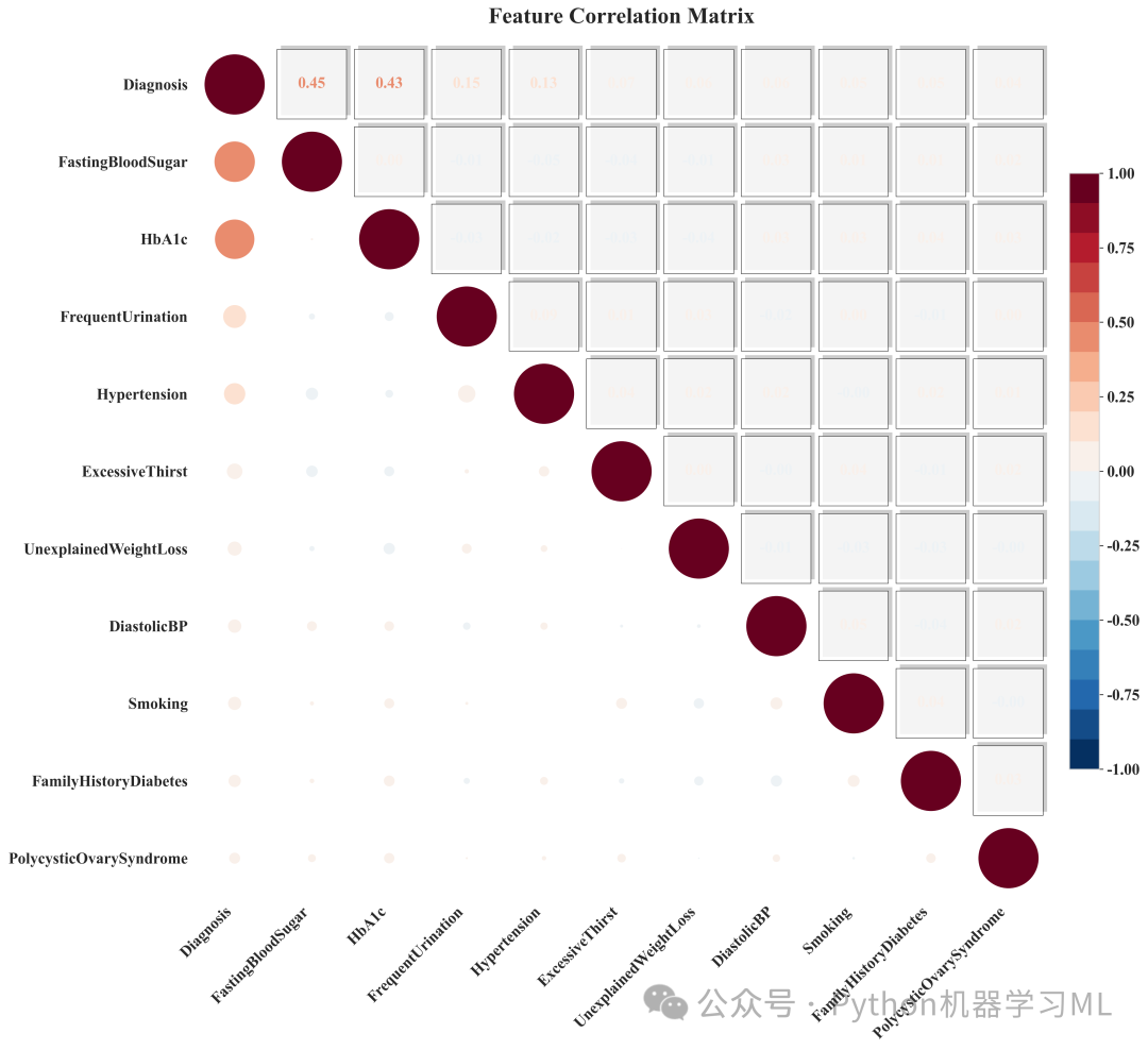
此阶段旨在量化特征之间的线性关系,特别是各个特征与目标变量Diagnosis之间的关系。
作用解释:
- 计算相关性矩阵
使用
.corr()计算所有数值特征之间的皮尔逊相关系数,系数范围从-1(完全负相关)到+1(完全正相关),0表示无线性关系。 - 目标相关性排序
提取每个特征与
Diagnosis的相关性,并按降序排列。这直接回答了“哪些特征与患病存在最强的线性关系?”这个问题,是初步筛选特征的有效方法。 - 热力图可视化
-
通过
seaborn.heatmap将复杂的相关性矩阵可视化。 mask=np.triu(...)是一个巧妙的技巧,它创建了一个上三角矩阵的掩码,使得热力图只显示下三角部分,避免了信息冗余,使图像更简洁。
cmap='coolwarm'是一个发散型色板,红色表示正相关,蓝色表示负相关,白色表示接近0,非常直观。
-
这个分析有助于识别高度相关的特征(可能存在多重共线性问题)和与目标强相关的特征。
# ==================== 第三部分:特征相关性分析 ====================
print("\n" + "=" * 70)
print("🔥 第三部分:特征相关性分析")
print("=" * 70)

correlation_matrix = data[numeric_cols + ['Diagnosis']].corr()
target_corr = correlation_matrix['Diagnosis'].sort_values(ascending=False)

print("\n🏆 与诊断结果相关性 Top 15:")
top15_corr = target_corr.head(16)[1:]
for i, (feature, corr) inenumerate(top15_corr.items(), 1):
print(f"  {i:2d}. {feature:30s}: {corr:+.4f}")

target_corr_df = pd.DataFrame({'Feature': target_corr.index, 'Correlation': target_corr.values})
target_corr_df.to_csv(f'{output_dir}/target_correlation.csv', index=False)

# 热力图
plt.figure(figsize=(18, 16))
mask = np.triu(np.ones_like(correlation_matrix, dtype=bool))
sns.heatmap(correlation_matrix, mask=mask, annot=False, cmap='coolwarm',
            center=0, linewidths=0.5, cbar_kws={'label': '相关系数'},
            square=True, vmin=-1, vmax=1)
plt.title('特征相关性矩阵(下三角)', fontsize=16, fontweight='bold', pad=20)
plt.tight_layout()
plt.savefig(f'{output_dir}/03_correlation_heatmap.png', dpi=300, bbox_inches='tight')
plt.show()
print(f"✅ 图表已保存: {output_dir}/03_correlation_heatmap.png")
阶段 4: 特征重要性分析 (互信息法)
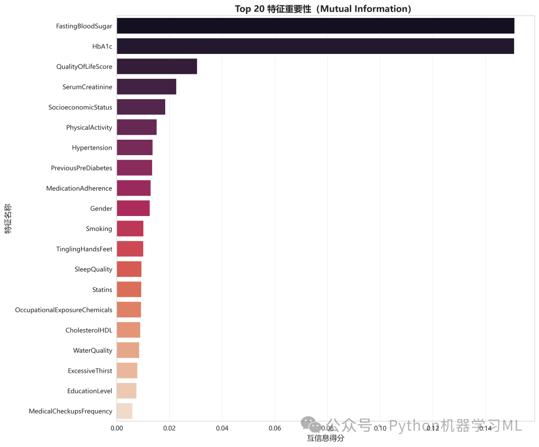
这个阶段采用互信息 (Mutual Information)来评估特征的重要性,这是一种比相关性更强大的方法。
作用解释:
- 什么是互信息
互信息能够衡量一个变量中包含的关于另一个变量的信息量。与只能捕捉线性关系的相关系数不同,互信息可以捕捉任何类型的统计依赖关系(包括线性和非线性)。得分越高,表示该特征与目标变量的关联性越强。
- 计算与排序
使用
sklearn.feature_selection.mutual_info_classif计算每个特征与目标Diagnosis之间的互信息得分。然后将得分从高到低排序,得到一个基于信息论的特征重要性排名。 - 可视化
通过条形图展示了互信息得分最高的20个特征,使得最重要的特征一目了然。
这是一个非常有效的、不依赖于任何特定模型的特征筛选方法。
python
# 第四部分:特征重要性分析(互信息法)==
print("\n" + "=" * 70)
print("🔗 第四部分:特征重要性分析(互信息法)")
print("=" * 70)

# 准备数据
features_for_analysis = [col for col in data.columns if col notin ['PatientID', 'Diagnosis']]
X = data[features_for_analysis]
y = data['Diagnosis']

# 计算互信息
print("\n⏳ 正在计算互信息得分...")
mi_scores = mutual_info_classif(X, y, random_state=42)
mi_df = pd.DataFrame({
'Feature': features_for_analysis,
'MI_Score': mi_scores
}).sort_values('MI_Score', ascending=False)

# 保存结果
mi_df.to_csv(f'{output_dir}/mutual_information_scores.csv', index=False)

print("\n🏆 Top 15 重要特征(互信息法):")
for i, row in mi_df.head(15).iterrows():
print(f"  {i+1:2d}. {row['Feature']:30s}: {row['MI_Score']:.6f}")

# 可视化 Top 20
plt.figure(figsize=(12, 10))
top20_mi = mi_df.head(20)
sns.barplot(data=top20_mi, y='Feature', x='MI_Score', palette='rocket')
plt.title('Top 20 特征重要性(Mutual Information)', fontsize=14, fontweight='bold')
plt.xlabel('互信息得分', fontsize=12)
plt.ylabel('特征名称', fontsize=12)
plt.grid(axis='x', alpha=0.3)
plt.tight_layout()
plt.savefig(f'{output_dir}/05_mutual_information_top20.png', dpi=300, bbox_inches='tight')
plt.show()
print(f"✅ 图表已保存: {output_dir}/05_mutual_information_top20.png")
阶段 5: 异常值检测
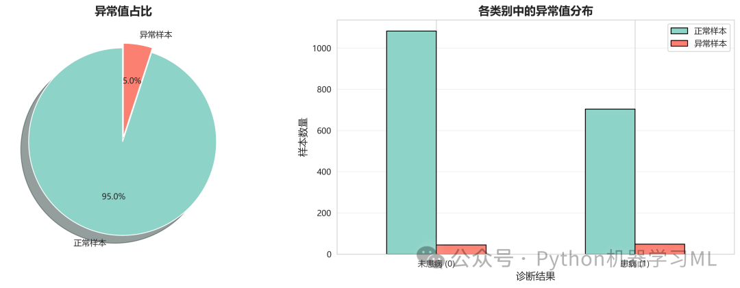
这个阶段使用一种多变量统计方法来识别数据集中的异常样本。
作用解释:
- 检测方法
代码使用了
sklearn.covariance.EllipticEnvelope(椭圆包络)。该方法假设“正常”的数据点服从一个高斯分布,它会尝试拟合一个椭圆来包围这些正常点,而位于椭圆之外的点则被认为是异常值。 - 标准化
在检测前对数据进行了标准化(
StandardScaler),这是非常重要的一步,因为EllipticEnvelope对特征的尺度很敏感。 contamination参数这个参数告诉算法数据集中异常值的大致比例(这里设为5%)。这是一个需要根据先验知识或业务理解调整的超参数。
- 分析与决策
代码不仅检测了异常值,还通过交叉表(
pd.crosstab)和可视化分析了异常值在不同诊断类别中的分布。它提供了一个开关REMOVE_OUTLIERS,允许用户选择是保留还是移除这些异常值。代码默认选择标记但不移除,可自行修改,这是一个稳健的做法,鼓励用户在删除数据前先进行深入分析。
python
# ==================== 第五部分:异常值检测 ====================
print("\n" + "=" * 70)
print("🔍 第五部分:异常值检测")
print("=" * 70)

defdetect_outliers(X, contamination=0.05):
"""使用椭圆包络检测多变量异常值"""
    detector = EllipticEnvelope(contamination=contamination, random_state=42)
    outlier_labels = detector.fit_predict(X)
    outlier_mask = outlier_labels == 1# 1表示正常,-1表示异常
    n_outliers = np.sum(~outlier_mask)
print(f"  检测到 {n_outliers} 个异常样本 (contamination={contamination}, 占比 {n_outliers/len(X)*100:.2f}%)")
return outlier_mask, outlier_labels

# 标准化后检测
print("\n⏳ 正在进行异常值检测...")
scaler = StandardScaler()
X_scaled = scaler.fit_transform(X)
outlier_mask, outlier_labels = detect_outliers(X_scaled, contamination=0.05)

# 标记异常值
data['Is_Outlier'] = ~outlier_mask

# 异常值分布统计
outlier_stats = pd.crosstab(data['Diagnosis'], data['Is_Outlier'], margins=True)
print("\n📊 异常值在各类别中的分布:")
print(outlier_stats)

# 可视化异常值分布
fig, axes = plt.subplots(1, 2, figsize=(14, 5))
outlier_counts = data['Is_Outlier'].value_counts()

# 饼图
axes[0].pie(
    outlier_counts,
    labels=['正常样本', '异常样本'],
    autopct='%1.1f%%',
    startangle=90,
    colors=['#8dd3c7', '#fb8072'],
    explode=(0.05, 0),
    shadow=True
)
axes[0].set_title('异常值占比', fontsize=14, fontweight='bold')

# 分组柱状图
outlier_by_diagnosis = data.groupby(['Diagnosis', 'Is_Outlier']).size().unstack(fill_value=0)
outlier_by_diagnosis.plot(kind='bar', ax=axes[1], color=['#8dd3c7', '#fb8072'], edgecolor='black')
axes[1].set_title('各类别中的异常值分布', fontsize=14, fontweight='bold')
axes[1].set_xlabel('诊断结果', fontsize=12)
axes[1].set_ylabel('样本数量', fontsize=12)
axes[1].set_xticklabels(['未患病 (0)', '患病 (1)'], rotation=0)
axes[1].legend(['正常样本', '异常样本'], loc='upper right')
axes[1].grid(axis='y', alpha=0.3)

plt.tight_layout()
plt.savefig(f'{output_dir}/06_outlier_detection.png', dpi=300, bbox_inches='tight')
plt.show()
print(f"✅ 图表已保存: {output_dir}/06_outlier_detection.png")

# 是否移除异常值
REMOVE_OUTLIERS = False
if REMOVE_OUTLIERS:
    data_clean = data[outlier_mask].copy()
print(f"\n✅ 已移除异常值,剩余样本数: {data_clean.shape[0]}")
print(f"   移除了 {data.shape[0] - data_clean.shape[0]} 个样本")
else:
    data_clean = data.copy()
print("\n⚠️ 保留所有样本(异常值已标记在 'Is_Outlier' 列)")
print("   建议:先观察异常样本特征,再决定是否移除")

data_clean.to_csv(f'{output_dir}/data_with_outlier_labels.csv', index=False)
print(f"✅ 标记数据已保存: {output_dir}/data_with_outlier_labels.csv")
阶段 6: 特征重要性分析 (Lasso法)
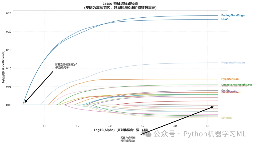
这个阶段引入了第三种特征重要性评估方法——Lasso回归。这是一种基于模型的强大特征选择技术。
作用解释:
- Lasso回归的原理
Lasso(Least Absolute Shrinkage and Selection Operator)是一种线性回归的变体,它在损失函数中加入了L1正则化项。这个正则化项会惩罚系数的绝对值,其效果是:当惩罚力度足够大时,许多不重要的特征的系数会被直接压缩到零,从而实现了自动的特征选择。
- Lasso路径图 (
lasso_path)这张图可视化了Lasso的特征选择过程。X轴
-log10(alpha),alpha是惩罚力度。从左到右,惩罚力度由强变弱。在最左侧(惩罚最强),所有系数都为0。随着向右移动(惩罚减弱),一些特征的系数开始脱离0线。越早脱离0线的特征,被认为越重要,因为它们在强惩罚下依然能对模型做出贡献。 - Lasso重要性得分
代码通过计算路径中系数绝对值的总和来为每个特征赋予一个单一的重要性得分,并用条形图展示了Top 10。
Lasso方法不仅能评估重要性,还能直接用于构建一个稀疏的(只使用少数特征的)预测模型。
# 1. 准备数据 (Lasso 对数据缩放非常敏感,必须标准化)
print("⏳ 正在标准化数据并计算 Lasso 路径...")
# 使用前面定义的 X 和 y
X_sample = X
y_target = y
feature_names_for_shap = features_for_analysis

scaler = StandardScaler()
X_scaled = scaler.fit_transform(X_sample)

# 2. 计算 Lasso 路径
alphas_lasso, coefs_lasso, _ = lasso_path(X_scaled, y_target, eps=0.001, n_alphas=100)

# 3. 绘图配置
plt.figure(figsize=(14, 8))
colors = plt.cm.tab20(np.linspace(0, 1, len(feature_names_for_shap)))

# 4. 绘制每一条特征的路径
log_alphas = -np.log10(alphas_lasso)
for i inrange(len(feature_names_for_shap)):
    plt.plot(log_alphas, coefs_lasso[i], color=colors[i], linewidth=1.5, alpha=0.8)

# 5. 寻找最重要的特征进行标注
final_coefs = np.abs(coefs_lasso[:, -1])
top_indices = np.argsort(final_coefs)[-10:]
for i in top_indices:
    feature_name = feature_names_for_shap[i]
    final_val = coefs_lasso[i, -1]
    plt.text(log_alphas[-1] + 0.05, final_val, feature_name,
             fontsize=10, fontweight='bold', color=colors[i], va='center')

# 6. 修正坐标轴与标题
plt.xlabel('-Log10(Alpha)  [正则化强度:强-->弱]', fontsize=12, fontweight='bold')
plt.ylabel('特征系数 (Coefficients)', fontsize=12)
plt.title('Lasso 特征选择路径图\n(左侧为高惩罚区,越早脱离0线的特征越重要)', fontsize=14, fontweight='bold')
plt.grid(which='both', linestyle='--', alpha=0.3)
plt.axhline(0, color='black', linewidth=1, linestyle='-')

plt.tight_layout()
save_path = f'{output_dir}/07_lasso_path.png'
plt.savefig(save_path, dpi=300, bbox_inches='tight')
plt.show()
print(f"✅ Lasso 路径图已保存: {save_path}")

# 计算Lasso重要性得分
features_for_lasso = feature_names_for_shap
feature_importance = np.sum(np.abs(coefs_lasso), axis=1)
sorted_top10 = np.argsort(feature_importance)[-10:]

# Lasso Top 10 可视化
lasso_top10_df = pd.DataFrame({
'Feature': [features_for_lasso[i] for i in sorted_top10],
'Importance': [feature_importance[i] for i in sorted_top10]
})
plt.figure(figsize=(12, 8))
sns.barplot(data=lasso_top10_df.sort_values('Importance', ascending=False), y='Feature', x='Importance', palette='viridis')
plt.title('Lasso 分析 - Top 10 最重要特征', fontsize=14, fontweight='bold')
plt.xlabel('重要性得分(系数绝对值总和)', fontsize=12)
plt.ylabel('特征名称', fontsize=12)
plt.grid(axis='x', alpha=0.3)
plt.tight_layout()
plt.savefig(f'{output_dir}/08_lasso_top10_features.png', dpi=300, bbox_inches='tight')
plt.show()
print(f"✅ 图表已保存: {output_dir}/08_lasso_top10_features.png")

lasso_importance_df = pd.DataFrame({
'Feature': features_for_lasso,
'Lasso_Importance': feature_importance
}).sort_values('Lasso_Importance', ascending=False)
lasso_importance_df.to_csv(f'{output_dir}/lasso_feature_importance.csv', index=False)
print(f"✅ Lasso 特征重要性已保存: {output_dir}/lasso_feature_importance.csv")
阶段 7: 综合特征重要性对比
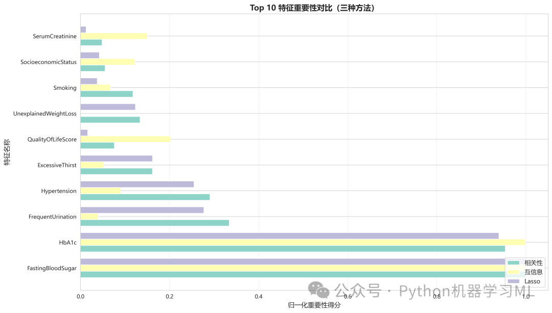
这是整个分析的点睛之笔。它将前面三种不同方法(相关性、互信息、Lasso)得到的重要性得分进行汇总,得出一个更稳健、更可靠的“综合排名”。
作用解释:
- 整合数据
将三种方法计算出的重要性得分合并到一个DataFrame中。
- 归一化处理
不同方法的得分尺度差异很大(例如,相关性在0-1之间,互信息和Lasso得分可能更大)。为了公平比较,代码使用
MinMaxScaler将所有得分都缩放到0到1的相同区间内。这是一个关键步骤。 - 计算综合得分
将归一化后的三个得分取平均值,得到一个“综合得分”。这个得分综合考虑了特征的线性关系、非线性关系以及在正则化模型中的表现。
- 最终排名与可视化
根据综合得分对特征进行最终排序,并用分组条形图可视化Top 10特征在三种方法下的不同表现。
这种综合评估的方法比依赖单一指标更科学,得出的结论也更有说服力。
python
#  第七部分:综合特征重要性对比
print("\n" + "=" * 70)
print("🏆 第七部分:综合特征重要性对比")
print("=" * 70)

corr_importance = target_corr.abs().to_frame('Correlation_Abs')
corr_importance.index.name = 'Feature'
corr_importance = corr_importance.reset_index()
corr_importance = corr_importance[corr_importance['Feature'] != 'Diagnosis']

combined = corr_importance.merge(mi_df, on='Feature', how='outer')
combined = combined.merge(lasso_importance_df, on='Feature', how='outer')
combined = combined.fillna(0)

scaler_norm = MinMaxScaler()
combined[['Correlation_Norm', 'MI_Norm', 'Lasso_Norm']] = scaler_norm.fit_transform(
    combined[['Correlation_Abs', 'MI_Score', 'Lasso_Importance']]
)

combined['综合得分'] = combined[['Correlation_Norm', 'MI_Norm', 'Lasso_Norm']].mean(axis=1)
combined = combined.sort_values('综合得分', ascending=False)
combined.to_csv(f'{output_dir}/combined_feature_importance.csv', index=False)
print(f"✅ 综合特征重要性已保存: {output_dir}/combined_feature_importance.csv")

print("\n🥇 综合评分 Top 15 特征:")
for i, row in combined.head(15).iterrows():
print(f"  {i+1:2d}. {row['Feature']:30s}: {row['综合得分']:.4f}")

# 可视化对比
top10_combined = combined.head(10)
fig, ax = plt.subplots(figsize=(14, 8))
x = np.arange(len(top10_combined))
width = 0.25

ax.barh(x - width, top10_combined['Correlation_Norm'], width, label='相关性', color='#8dd3c7')
ax.barh(x, top10_combined['MI_Norm'], width, label='互信息', color='#ffffb3')
ax.barh(x + width, top10_combined['Lasso_Norm'], width, label='Lasso', color='#bebada')

ax.set_xlabel('归一化重要性得分', fontsize=12)
ax.set_ylabel('特征名称', fontsize=12)
ax.set_title('Top 10 特征重要性对比(三种方法)', fontsize=14, fontweight='bold')
ax.set_yticks(x)
ax.set_yticklabels(top10_combined['Feature'])
ax.legend(loc='lower right', fontsize=11)
ax.grid(axis='x', alpha=0.3)

plt.tight_layout()
plt.savefig(f'{output_dir}/09_combined_importance_comparison.png', dpi=300, bbox_inches='tight')
plt.show()
print(f"✅ 图表已保存: {output_dir}/09_combined_importance_comparison.png")
阶段 8: 数据准备与特征工程
在完成了探索性数据分析和特征重要性评估后,这个阶段正式开始为机器学习建模准备数据。
作用解释:
- 特征选择
代码提供了一个开关
USE_TOP_FEATURES。当它为True时,会根据上一阶段计算出的综合重要性排名,选择前N(这里是30)个特征,可结合自己数据集实际情况进行修改调整。这是一个非常关键的步骤,它利用了前面所有分析的成果,旨在通过减少特征数量来降低模型复杂度、减少过拟合风险并可能提升训练速度。 - 数据构建
基于选择的特征,创建了最终用于建模的
X_model和y_model。 - 可选的特征工程(是否创建交互式特征)
代码中包含了交互特征创建部分 (
CREATE_INTERACTION),本项目是False。它的作用是选取最重要的几个特征,将它们两两相乘,生成新的“交互特征”。例如,Age * BMI可能比单独的Age或BMI更能捕捉某些复杂的生理关系。这是一种高级的特征工程手段,通常在特征数量不多时尝试,以增强模型的表达能力。
python
#  第八部分:数据准备与特征工程 ====================
print("\n" + "=" * 70)
print("🔧 第八部分:数据准备与特征工程")
print("=" * 70)

print("\n📌 当前数据状态:")
print(f"  • 样本数: {data_clean.shape[0]}")
print(f"  • 特征数: {len(features_for_analysis)}")

# 基于综合特征重要性选择Top特征
USE_TOP_FEATURES = True
TOP_N_FEATURES = 30

if USE_TOP_FEATURES:
    selected_features = combined.head(TOP_N_FEATURES)['Feature'].tolist()
print(f"\n✅ 选择 Top {TOP_N_FEATURES} 特征用于建模:")
for i, feat inenumerate(selected_features, 1):
print(f"  {i:2d}. {feat}")
else:
    selected_features = features_for_analysis
print(f"\n✅ 使用全部 {len(selected_features)} 个特征")

# 准备建模数据
X_model = data_clean[selected_features].copy()
y_model = data_clean['Diagnosis'].copy()
print(f"\n📊 建模数据维度: X={X_model.shape}, y={y_model.shape}")
print(f"   类别分布: {dict(y_model.value_counts())}")

# 可选交互特征
CREATE_INTERACTION = False
if CREATE_INTERACTION andlen(selected_features) <= 15:
print("\n🔨 正在创建交互特征...")
    key_for_interaction = selected_features[:5]
for i inrange(len(key_for_interaction)):
for j inrange(i + 1, len(key_for_interaction)):
            feat1, feat2 = key_for_interaction[i], key_for_interaction[j]
            new_feat_name = f"{feat1}_x_{feat2}"
            X_model[new_feat_name] = X_model[feat1] * X_model[feat2]
print(f"✅ 创建了 {len(X_model.columns) - len(selected_features)} 个交互特征")
print(f"   当前特征总数: {X_model.shape[1]}")

feature_names = X_model.columns.tolist()
阶段 9: 数据划分
这个阶段将准备好的数据划分为训练集和测试集,这是评估模型泛化能力的标准做法。
作用解释:
train_test_split将数据集按照80/20的比例分割。
stratify=y_model这是此步骤中最关键的参数。由于我们的目标变量类别不平衡,使用分层抽样可以确保训练集和测试集中的“患病”与“未患病”样本比例与原始数据集保持一致。这避免了因随机划分导致某个集合中某种类别样本过少而影响模型训练和评估的公正性。
python
# ==================== 第九部分:数据划分 ====================
print("\n" + "=" * 70)
print("✂️ 第九部分:数据划分")
print("=" * 70)

TEST_SIZE = 0.2
RANDOM_STATE = 42

X_train, X_test, y_train, y_test = train_test_split(
    X_model, y_model,
    test_size=TEST_SIZE,
    random_state=RANDOM_STATE,
    stratify=y_model
)

print("\n📊 数据划分结果:")
print(f"  • 训练集: {X_train.shape[0]} 样本 ({X_train.shape[0] / len(X_model) * 100:.1f}%)")
print(f"  • 测试集: {X_test.shape[0]} 样本 ({X_test.shape[0] / len(X_model) * 100:.1f}%)")
print(f"  训练集类别分布: {dict(y_train.value_counts())}")
print(f"  测试集类别分布: {dict(y_test.value_counts())}")
阶段 10: 动态建模管道与超参数空间定义
这是整个代码最核心和最复杂的部分,它定义了一个高度灵活的自动化建模框架。
作用解释:
get_model_with_params这是一个模型“工厂”函数。它接收一个模型名称和Optuna的
trial对象,然后返回一个具体的模型实例。trial.suggest_*系列函数定义了每个模型需要优化的超参数及其搜索范围(例如,随机森林的n_estimators在100到500之间搜索)。create_advanced_pipeline这是一个极其强大的“管道”构建函数。它允许Optuna在优化过程中动态地组合不同的预处理步骤,实现了类似AutoML(自动化机器学习)的功能。这个管道的步骤包括:
- 数据缩放
自动选择
StandardScaler(标准缩放)或RobustScaler(对异常值更稳健的缩放)。 - 类别不平衡处理
自动选择不处理、
SMOTE(合成少数类过采样)、ADASYN(自适应合成采样)或SMOTEENN(结合过采样和欠采样)。 - 特征选择
自动选择不处理、
SelectKBest(选择最好的K个特征)、RFE(递归特征消除)或基于Lasso的SelectFromModel。 - 多项式特征
可选地创建交互特征。
- 模型
最后一步是模型本身。
- 数据缩放
通过这种方式,Optuna不仅在寻找最佳的模型参数,还在寻找最佳的预处理流程组合,大大提升了找到最优解的可能性。
python
# 第十部分:模型定义与参数空间 ====================
print("\n" + "=" * 70)
print("🎯 第十部分:模型定义与超参数空间")
print("=" * 70)

cv = StratifiedKFold(n_splits=5, shuffle=True, random_state=RANDOM_STATE)


defget_model_with_params(model_name, trial):
"""根据模型名称和trial返回模型实例"""
if model_name == "Logistic Regression":
        penalty = trial.suggest_categorical('penalty', ['l1', 'l2', 'elasticnet'])
        params = {
'C': trial.suggest_float('C', 0.01, 100, log=True),
'penalty': penalty,
'solver': 'saga',
'max_iter': 1000,
'random_state': RANDOM_STATE
        }
if penalty == 'elasticnet':
            params['l1_ratio'] = trial.suggest_float('l1_ratio', 0, 1)
return LogisticRegression(**params)

elif model_name == "Random Forest":
return RandomForestClassifier(
            n_estimators=trial.suggest_int('n_estimators', 100, 500),
            max_depth=trial.suggest_int('max_depth', 5, 25),
            min_samples_split=trial.suggest_int('min_samples_split', 2, 20),
            min_samples_leaf=trial.suggest_int('min_samples_leaf', 1, 10),
            max_features=trial.suggest_categorical('max_features', ['sqrt', 'log2', None]),
            bootstrap=trial.suggest_categorical('bootstrap', [True, False]),
            random_state=RANDOM_STATE,
            n_jobs=-1
        )

elif model_name == "Gradient Boosting":
return GradientBoostingClassifier(
            n_estimators=trial.suggest_int('n_estimators', 50, 500),
            learning_rate=trial.suggest_float('learning_rate', 0.01, 0.3),
            max_depth=trial.suggest_int('max_depth', 3, 10),
            subsample=trial.suggest_float('subsample', 0.6, 1.0),
            min_samples_split=trial.suggest_int('min_samples_split', 2, 20),
            random_state=RANDOM_STATE
        )

elif model_name == "XGBoost":
return XGBClassifier(
            n_estimators=trial.suggest_int('n_estimators', 50, 500),
            learning_rate=trial.suggest_float('learning_rate', 0.01, 0.3),
            max_depth=trial.suggest_int('max_depth', 3, 10),
            subsample=trial.suggest_float('subsample', 0.6, 1.0),
            colsample_bytree=trial.suggest_float('colsample_bytree', 0.6, 1.0),
            reg_alpha=trial.suggest_float('reg_alpha', 0, 10),
            reg_lambda=trial.suggest_float('reg_lambda', 0, 10),
            eval_metric='logloss',
            random_state=RANDOM_STATE,
            n_jobs=-1
        )

elif model_name == "LightGBM":
return LGBMClassifier(
            n_estimators=trial.suggest_int('n_estimators', 50, 500),
            learning_rate=trial.suggest_float('learning_rate', 0.01, 0.3),
            num_leaves=trial.suggest_int('num_leaves', 10, 100),
            max_depth=trial.suggest_int('max_depth', 3, 15),
            feature_fraction=trial.suggest_float('feature_fraction', 0.6, 1.0),
            bagging_fraction=trial.suggest_float('bagging_fraction', 0.6, 1.0),
            reg_alpha=trial.suggest_float('reg_alpha', 0, 10),
            reg_lambda=trial.suggest_float('reg_lambda', 0, 10),
            random_state=RANDOM_STATE,
            verbose=-1,
            n_jobs=-1
        )

elif model_name == "MLP":
        hidden_size_1 = trial.suggest_int('hidden_size_1', 50, 200)
        hidden_size_2 = trial.suggest_int('hidden_size_2', 20, 100)
return MLPClassifier(
            hidden_layer_sizes=(hidden_size_1, hidden_size_2),
            alpha=trial.suggest_float('alpha', 1e-5, 1e-1, log=True),
            learning_rate_init=trial.suggest_float('learning_rate_init', 1e-4, 1e-1, log=True),
            activation=trial.suggest_categorical('activation', ['tanh', 'relu']),
            max_iter=500,
            early_stopping=True,
            random_state=RANDOM_STATE
        )

elif model_name == "AdaBoost":
return AdaBoostClassifier(
            n_estimators=trial.suggest_int('n_estimators', 50, 500),
            learning_rate=trial.suggest_float('learning_rate', 0.01, 2.0),
            random_state=RANDOM_STATE
        )

elif model_name == "ExtraTrees":
return ExtraTreesClassifier(
            n_estimators=trial.suggest_int('n_estimators', 100, 500),
            max_depth=trial.suggest_int('max_depth', 5, 25),
            min_samples_split=trial.suggest_int('min_samples_split', 2, 20),
            min_samples_leaf=trial.suggest_int('min_samples_leaf', 1, 10),
            max_features=trial.suggest_categorical('max_features', ['sqrt', 'log2', None]),
            bootstrap=trial.suggest_categorical('bootstrap', [True, False]),
            random_state=RANDOM_STATE,
            n_jobs=-1
        )

elif model_name == "Naive Bayes":
return GaussianNB(
            var_smoothing=trial.suggest_float('var_smoothing', 1e-10, 1e-6, log=True)
        )


defcreate_advanced_pipeline(model_name, trial, X_train, y_train):
"""创建包含预处理、采样和模型的完整Pipeline"""
    steps = []

# 1. 数据缩放
    scaler_type = trial.suggest_categorical('scaler', ['standard', 'robust'])
if scaler_type == 'standard':
        steps.append(('scaler', StandardScaler()))
else:
        steps.append(('scaler', RobustScaler()))

# 2. 处理类别不平衡
    sampling_method = trial.suggest_categorical('sampling', ['none', 'smote', 'adasyn', 'smoteenn'])
    min_class_samples = min(np.sum(y_train == 0), np.sum(y_train == 1))
    k_neighbors = min(5, min_class_samples - 1)

if sampling_method == 'smote':
        steps.append(('sampler', SMOTE(random_state=RANDOM_STATE, k_neighbors=k_neighbors)))
elif sampling_method == 'adasyn':
        steps.append(('sampler', ADASYN(random_state=RANDOM_STATE, n_neighbors=k_neighbors)))
elif sampling_method == 'smoteenn':
        steps.append(('sampler', SMOTEENN(random_state=RANDOM_STATE)))

# 3. 特征选择(省略,私信作者,微信:zyfxw888)


# 4. 可选多项式特征
if X_train.shape[1] <= 20:
if trial.suggest_categorical('poly_features', [False, True]):
            degree = trial.suggest_int('poly_degree', 2, 2)
            steps.append(('poly', PolynomialFeatures(
                degree=degree,
                interaction_only=True,
                include_bias=False
            )))

# 5. 模型
    model = get_model_with_params(model_name, trial)
    steps.append(('model', model))

if sampling_method != 'none':
return ImbPipeline(steps)
else:
return Pipeline(steps)


print("\n✅ 模型参数空间定义完成")
print("   支持的模型: Logistic Regression, Random Forest, Gradient Boosting,")
print("              XGBoost, LightGBM, MLP, AdaBoost, ExtraTrees, Naive Bayes")
阶段 11: 使用Optuna进行超参数优化
此阶段利用Optuna框架,自动化地为我们定义的多个模型寻找最佳的超参数组合。
作用解释:
objective_function这是优化的核心,是Optuna需要最大化(或最小化)的目标。它接收一个
trial对象,通过create_advanced_pipeline构建一个完整的建模流程,然后使用5折交叉验证(cross_val_score)在训练集上评估这个流程的性能(以roc_auc为指标)。返回的平均分就是本次“试验”的得分。optuna.create_study创建一个优化任务。
direction='maximize'表示我们希望roc_auc得分越高越好。- Sampler (TPESampler)
这是一个智能采样器,它会根据历史试验的结果,更有可能在表现好的参数区域进行下一次采样。
- Pruner (MedianPruner)
这是一个剪枝器,用于提前终止那些早期表现不佳的试验,从而节省大量计算时间。
- Sampler (TPESampler)
- 循环优化
代码遍历预定义的模型列表,为每个模型运行一次完整的优化过程(
study.optimize)。 - 结果存储
对每个模型,都保存了最佳的交叉验证分数、最佳参数组合以及训练好的最佳管道(
optimized_models)。
这个过程免去了手动调参的繁琐和盲目性,能够系统性地探索巨大的参数空间。
python
# 第十一部分:Optuna 超参数优化 ====================
print("\n" + "=" * 70)
print("🔍 第十一部分:使用 Optuna 进行超参数优化")
print("=" * 70)


defobjective_function(trial, model_name, X_train, y_train, cv):
"""Optuna优化目标函数"""
try:
        pipeline = create_advanced_pipeline(model_name, trial, X_train, y_train)
        scores = cross_val_score(
            pipeline, X_train, y_train,
            cv=cv,
            scoring='roc_auc',
            n_jobs=-1
        )
        mean_score = np.mean(scores)
if np.isnan(mean_score):
return0.0
return mean_score
except Exception as e:
return0.0


model_names = [
"Logistic Regression",
"Random Forest",
"Gradient Boosting",
"XGBoost",
"LightGBM",
"MLP",
"AdaBoost",
"ExtraTrees",
"Naive Bayes"
]

optimized_models = {}
best_params_dict = {}
optimization_results = {}

print(f"\n🎯 开始优化 {len(model_names)} 个模型...\n")

for idx, model_name inenumerate(model_names, 1):
print("=" * 60)
print(f"[{idx}/{len(model_names)}] 正在优化: {model_name}")
print("=" * 60)

    start_time = time.time()
    sampler = TPESampler(seed=RANDOM_STATE)
    pruner = MedianPruner(n_startup_trials=5, n_warmup_steps=3)

    study = optuna.create_study(
        direction='maximize',
        sampler=sampler,
        pruner=pruner
    )

if model_name in ["MLP", "XGBoost", "LightGBM"]:
        n_trials = 60
else:
        n_trials = 40

    study.optimize(
lambda trial: objective_function(trial, model_name, X_train, y_train, cv),
        n_trials=n_trials,
        timeout=600,
        show_progress_bar=False
    )

    best_params = study.best_params
    best_params_dict[model_name] = best_params

    best_pipeline = create_advanced_pipeline(model_name, study.best_trial, X_train, y_train)
    best_pipeline.fit(X_train, y_train)
    optimized_models[model_name] = best_pipeline

    optimization_results[model_name] = {
'best_score': study.best_value,
'n_trials': len(study.trials),
'best_params': best_params,
'optimization_time': time.time() - start_time
    }

print(f"\n✅ 优化完成!")
print(f"   最佳 AUC (CV): {study.best_value:.4f}")
print(f"   优化时间: {time.time() - start_time:.1f} 秒")
print(f"   试验次数: {len(study.trials)}")

    key_params = {k: v for k, v in best_params.items()
if k in ['scaler', 'sampling', 'feature_selection']}
print(f"   关键配置: {key_params}")
print()
阶段 12: 单模型性能评估与对比
这是“验收”阶段。在通过交叉验证找到了每个模型的最佳配置后,我们在从未见过的测试集上评估它们的最终性能。
作用解释:
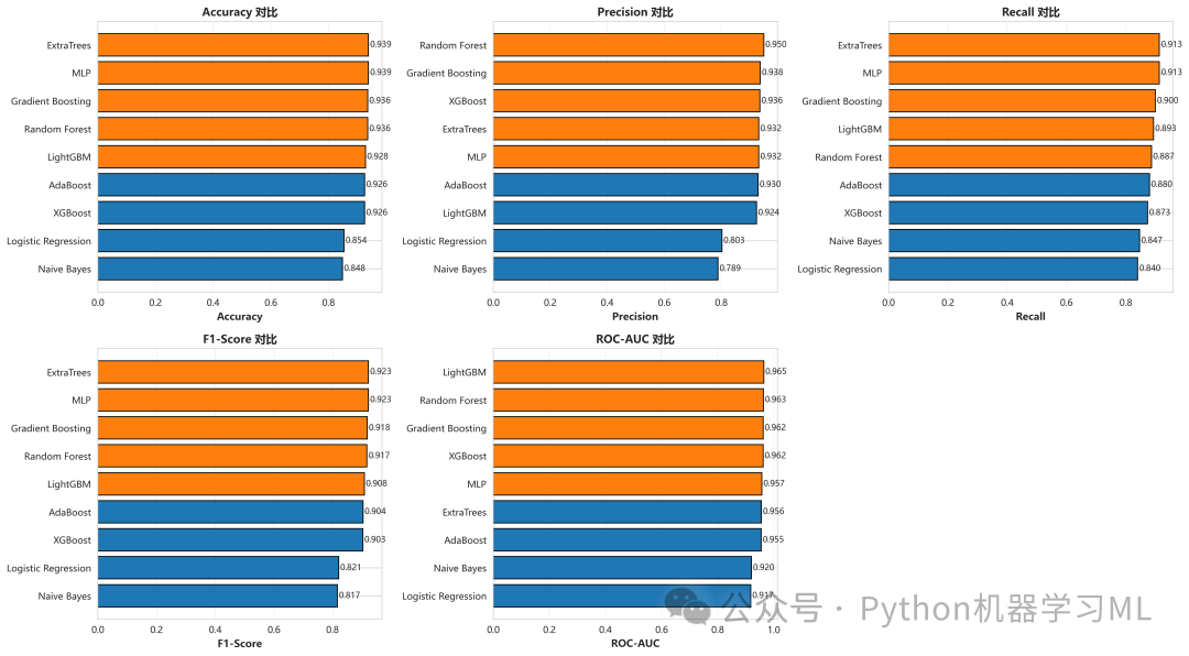
evaluate_model这个函数在测试集上计算了一系列关键的分类指标:
- Accuracy
准确率(预测正确的比例)。
- Precision
精确率(预测为正的样本中,真正为正的比例)。
- Recall
召回率(所有正样本中,被成功预测为正的比例)。
- F1-Score
精确率和召回率的调和平均数,是综合评价的常用指标。
- ROC-AUC
衡量模型区分正负样本能力的指标,对类别不平衡不敏感,是本次优化的核心指标。
- Accuracy
- 最终评估
代码遍历所有优化好的模型,在测试集上运行评估,并将结果汇总到一个DataFrame中,按ROC-AUC排序。
- 可视化
通过条形图直观地对比了不同模型在各项指标上的表现,使得哪个模型综合性能更优一目了然。
这个阶段的结果为我们选择最终部署哪个模型提供了最直接、最可靠的依据。
python
# ==================== 第十二部分:单模型性能评估 ====================
print("\n" + "=" * 70)
print("📊 第十二部分:单模型性能评估")
print("=" * 70)


defevaluate_model(model, X_test, y_test, model_name):
"""评估单个模型的性能"""
    y_pred = model.predict(X_test)
    y_pred_proba = model.predict_proba(X_test)[:, 1]

    metrics = {
'Model': model_name,
'Accuracy': accuracy_score(y_test, y_pred),
'Precision': precision_score(y_test, y_pred, zero_division=0),
'Recall': recall_score(y_test, y_pred, zero_division=0),
'F1-Score': f1_score(y_test, y_pred, zero_division=0),
'ROC-AUC': roc_auc_score(y_test, y_pred_proba)
    }

return metrics, y_pred, y_pred_proba


print("\n🔍 在测试集上评估所有模型...\n")
all_metrics = []
all_predictions = {}

for model_name, model in optimized_models.items():
    metrics, y_pred, y_pred_proba = evaluate_model(model, X_test, y_test, model_name)
    all_metrics.append(metrics)
    all_predictions[model_name] = {
'y_pred': y_pred,
'y_pred_proba': y_pred_proba
    }

results_df = pd.DataFrame(all_metrics)
results_df = results_df.sort_values('ROC-AUC', ascending=False)

print("📋 测试集性能对比:")
print(results_df.to_string(index=False))
print()

results_df.to_csv(f'{output_dir}/model_performance_comparison.csv', index=False)
print(f"✅ 性能对比已保存: {output_dir}/model_performance_comparison.csv")

# 可视化性能对比
fig, axes = plt.subplots(2, 3, figsize=(18, 10))
axes = axes.flatten()

metrics_to_plot = ['Accuracy', 'Precision', 'Recall', 'F1-Score', 'ROC-AUC']

for idx, metric inenumerate(metrics_to_plot):
    ax = axes[idx]
    data_sorted = results_df.sort_values(metric, ascending=True)
    colors_bars = ['#1f77b4'if x < data_sorted[metric].median() else'#ff7f0e'
for x in data_sorted[metric]]

    ax.barh(data_sorted['Model'], data_sorted[metric], color=colors_bars, edgecolor='black')
    ax.set_xlabel(metric, fontsize=11, fontweight='bold')
    ax.set_title(f'{metric} 对比', fontsize=12, fontweight='bold')
    ax.grid(axis='x', alpha=0.3)

for i, v inenumerate(data_sorted[metric]):
        ax.text(v + 0.005, i, f'{v:.3f}', va='center', fontsize=9)

axes[-1].axis('off')

plt.tight_layout()
plt.savefig(f'{output_dir}/10_model_performance_comparison.png', dpi=300, bbox_inches='tight')
plt.show()
print(f"✅ 图表已保存: {output_dir}/10_model_performance_comparison.png")
阶段 13: Stacking 集成模型构建与优化
这个阶段通过Stacking(堆叠)技术,尝试构建一个比任何单个模型都更强大的集成模型。
作用解释:
- 基本思想
Stacking 的核心思想是“学习如何组合模型”。它分为两层:
- 第一层(基学习器)
使用在上一阶段表现最好的4个单模型作为“基学习器”。
- 第二层(元学习器)
训练一个新的模型(称为“元模型”),这个模型的输入不再是原始数据,而是第一层所有基学习器对数据的预测结果。元模型的任务就是学习如何根据这些基模型的“意见”来做出最终、更准确的判断。
- 第一层(基学习器)
- 自动优化元模型
代码再次使用
Optuna来自动寻找最佳的元模型(是从逻辑回归、随机森林和XGBoost中选一个)以及其最优超参数。这确保了我们能找到最高效的组合方式。 - 评估与整合
优化后的Stacking模型被训练、评估,并将其性能指标添加到最终的排行榜中,与其他模型进行比较。
Stacking是一种强大的集成技术,常常能在数据科学竞赛中取得顶尖成绩。
python
#  第十三部分:创建 Stacking 集成模型 ====================
print("\n" + "=" * 70)
print("🏗️ 第十三部分:创建 Stacking 集成模型")
print("=" * 70)
(省略,私信作者,微信:zyfxw888)
print("\n🏆 选择的顶级基模型:")
 for i, (mn, score) inenumerate(top_models, 1):
 print(f"  {i}. {mn:25s} (AUC: {score:.4f})")

 base_learners = [(mn.replace(" ", "_").lower(), optimized_models[mn])
 for mn, _ in top_models]


 defcreate_stacking_classifier(trial):
 """创建Stacking集成分类器"""
     meta_model_name = trial.suggest_categorical('meta_model',
                                                 ['LogisticRegression', 'RandomForest', 'XGBoost'])

 if meta_model_name == 'LogisticRegression':
         meta_model = LogisticRegression(
             C=trial.suggest_float('meta_C', 0.01, 100, log=True),
             random_state=RANDOM_STATE,
             max_iter=1000
         )
 elif meta_model_name == 'RandomForest':
         meta_model = RandomForestClassifier(
             n_estimators=trial.suggest_int('meta_n_estimators', 50, 200),
             max_depth=trial.suggest_int('meta_max_depth', 3, 10),
             random_state=RANDOM_STATE,
             n_jobs=-1
         )
 else:
         meta_model = XGBClassifier(
             n_estimators=trial.suggest_int('meta_n_estimators', 50, 200),
             learning_rate=trial.suggest_float('meta_learning_rate', 0.01, 0.3),
             max_depth=trial.suggest_int('meta_max_depth', 3, 8),
             use_label_encoder=False,
             eval_metric='logloss',
             random_state=RANDOM_STATE,
             n_jobs=-1
         )

 return StackingClassifier(
         estimators=base_learners,
         final_estimator=meta_model,
         cv=3,
         passthrough=trial.suggest_categorical('passthrough', [True, False]),
         n_jobs=-1
     )


 print("\n🔧 正在优化 Stacking 集成模型...")
 stacking_study = optuna.create_study(direction='maximize', sampler=TPESampler(seed=RANDOM_STATE))


 defstacking_objective(trial):
 try:
         stacking_clf = create_stacking_classifier(trial)
         scores = cross_val_score(stacking_clf, X_train, y_train, cv=cv, scoring='roc_auc', n_jobs=-1)
 return np.mean(scores)
 except Exception as e:
 print(f"❌ Stacking 优化失败: {e}")
 return0.0


 start_time = time.time()
 stacking_study.optimize(stacking_objective, n_trials=20, timeout=300, show_progress_bar=False)
 stacking_time = time.time() - start_time

 print(f"\n✅ Stacking 优化完成!")
 print(f"   最佳 AUC (CV): {stacking_study.best_value:.4f}")
 print(f"   优化时间: {stacking_time:.1f} 秒")
 print(f"   最佳元模型: {stacking_study.best_params['meta_model']}")

 best_stacking_clf = create_stacking_classifier(stacking_study.best_trial)
 best_stacking_clf.fit(X_train, y_train)

 stacking_metrics, stacking_pred, stacking_proba = evaluate_model(
     best_stacking_clf, X_test, y_test, 'Stacking Ensemble'
 )

 print(f"\n📊 Stacking 模型测试集性能:")
 for key, value in stacking_metrics.items():
 if key != 'Model':
 print(f"   {key:12s}: {value:.4f}")

 optimized_models['Stacking Ensemble'] = best_stacking_clf
 all_predictions['Stacking Ensemble'] = {
 'y_pred': stacking_pred,
 'y_pred_proba': stacking_proba
 }

 results_df = pd.concat([results_df, pd.DataFrame([stacking_metrics])], ignore_index=True)
 results_df = results_df.sort_values('ROC-AUC', ascending=False)

 print("\n📋 更新后的性能对比(包含Stacking):")
 print(results_df.to_string(index=False))
阶段 14: 创建 Voting 集成模型
这是另一种强大的集成技术——投票法(Voting)。它比Stacking更简单,但同样非常有效。
作用解释:
- 基本思想
Voting集成的理念是“三个臭皮匠,顶个诸葛亮”。它将多个模型的预测结果结合起来,通过“投票”来决定最终结果。
voting='soft'(软投票)这是此处的关键。不同于“硬投票”(少数服从多数),软投票会计算所有基模型预测为某一类的平均概率。例如,如果三个模型预测样本A为“患病”的概率分别是0.9、0.6、0.8,软投票会计算平均概率(0.9+0.6+0.8)/3 = 0.77,然后基于这个概率做出决策。软投票通常比硬投票效果更好,因为它考虑了每个模型对其预测的“信心”程度。
python
# 第十四部分:创建 Voting 集成模型 ====================
print("\n" + "=" * 70)
print("🗳️ 第十四部分:创建 Voting 集成模型")
print("=" * 70)

voting_clf = VotingClassifier(
    estimators=base_learners,
    voting='soft',
    n_jobs=-1
)

print("\n⏳ 正在训练 Voting 集成模型...")
start_time = time.time()
voting_clf.fit(X_train, y_train)
voting_time = time.time() - start_time

voting_metrics, voting_pred, voting_proba = evaluate_model(
    voting_clf, X_test, y_test, 'Voting Ensemble'
)

print(f"\n✅ Voting 模型训练完成! (耗时: {voting_time:.1f} 秒)")
print(f"\n📊 Voting 模型测试集性能:")
for key, value in voting_metrics.items():
if key != 'Model':
print(f"   {key:12s}: {value:.4f}")

optimized_models['Voting Ensemble'] = voting_clf
all_predictions['Voting Ensemble'] = {
'y_pred': voting_pred,
'y_pred_proba': voting_proba
}

results_df = pd.concat([results_df, pd.DataFrame([voting_metrics])], ignore_index=True)
results_df = results_df.sort_values('ROC-AUC', ascending=False)

print("\n📋 最终性能对比(包含所有集成模型):")
print(results_df.to_string(index=False))

results_df.to_csv(f'{output_dir}/final_model_performance.csv', index=False)
print(f"\n✅ 最终结果已保存: {output_dir}/final_model_performance.csv")
阶段 15: ROC曲线对比
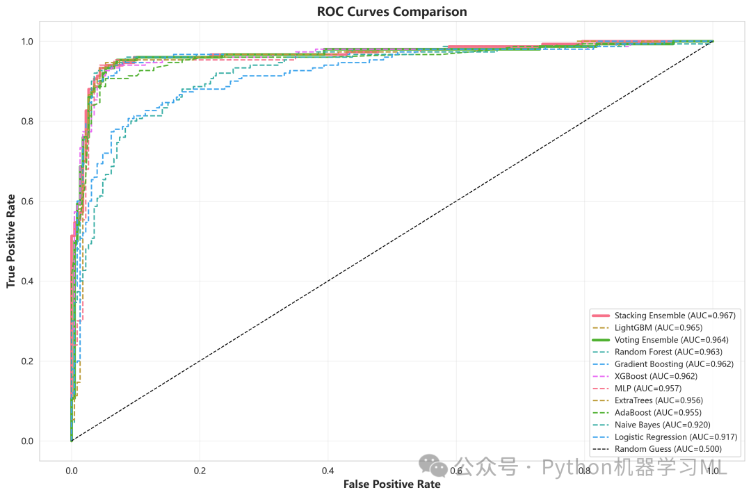
这个阶段将所有模型的性能通过ROC曲线进行可视化,提供了一个直观的全局比较。
作用解释:
- ROC曲线 (Receiver Operating Characteristic Curve)
横轴是“假阳性率”(FPR,把健康的误诊为患病),纵轴是“真阳性率”(TPR,成功诊断出患病,即召回率)。
- 解读
-
-
一个理想的模型会尽可能地靠近左上角(FPR=0, TPR=1)。
-
曲线越往左上方凸,说明模型在保持低误诊率的同时,能有更高的诊断率,性能越好。
- AUC (Area Under Curve)
ROC曲线下方的面积,是衡量模型整体性能的数值指标。AUC为1是完美模型,0.5则相当于随机猜测。
-
- 可视化效果
代码特意将集成模型(Stacking, Voting)的线条加粗,可以很清晰地看到,集成模型的曲线通常会包住大部分单模型,展示出其优越的综合性能。
python
# ============ 第十五部分:ROC曲线对比 ====================
print("\n" + "=" * 70)
print("📈 第十五部分:ROC 曲线可视化")
print("=" * 70)

plt.figure(figsize=(12, 8))

for model_name in results_df['Model']:
    y_pred_proba = all_predictions[model_name]['y_pred_proba']
    fpr, tpr, _ = roc_curve(y_test, y_pred_proba)
    auc_score = roc_auc_score(y_test, y_pred_proba)

    linewidth = 3if'Ensemble'in model_name else1.5
    linestyle = '-'if'Ensemble'in model_name else'--'

    plt.plot(fpr, tpr, label=f'{model_name} (AUC={auc_score:.3f})',
             linewidth=linewidth, linestyle=linestyle)

plt.plot([0, 1], [0, 1], 'k--', linewidth=1, label='Random Guess (AUC=0.500)')

plt.xlabel('False Positive Rate', fontsize=12, fontweight='bold')
plt.ylabel('True Positive Rate', fontsize=12, fontweight='bold')
plt.title('ROC Curves Comparison', fontsize=14, fontweight='bold')
plt.legend(loc='lower right', fontsize=9)
plt.grid(alpha=0.3)
plt.tight_layout()
plt.savefig(f'{output_dir}/11_roc_curves_comparison.png', dpi=300, bbox_inches='tight')
plt.show()
print(f"✅ ROC曲线已保存: {output_dir}/11_roc_curves_comparison.png")
阶段 16: 混淆矩阵可视化
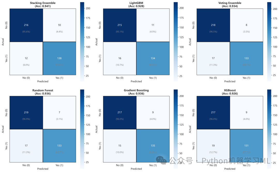
这个阶段为表现最好的6个模型绘制了混淆矩阵,以进行更深入的错误分析。
作用解释:
- 混淆矩阵 (Confusion Matrix)
它详细展示了模型预测的“混淆”情况。
- 左上 (TN)
实际为阴性,预测也为阴性(正确)。
- 右下 (TP)
实际为阳性,预测也为阳性(正确)。
- 右上 (FP)
实际为阴性,预测为阳性(假阳性,I类错误)。
- 左下 (FN)
实际为阳性,预测为阴性(假阴性,II类错误,通常是医疗场景中最危险的错误)。
- 左上 (TN)
- 深度分析
通过对比不同模型的混淆矩阵,我们可以分析它们的行为偏好。例如,某个模型的假阴性(FN)数量特别低,说明它在识别患者方面非常敏感,宁可“错杀”也不“放过”,这在某些应用场景下是至关重要的。
python
# ========== 第十六部分:混淆矩阵可视化 ====================
print("\n" + "=" * 70)
print("🔲 第十六部分:混淆矩阵可视化")
print("=" * 70)

top6_models = results_df.head(6)['Model'].tolist()

fig, axes = plt.subplots(2, 3, figsize=(16, 10))
axes = axes.flatten()

for idx, model_name inenumerate(top6_models):
    y_pred = all_predictions[model_name]['y_pred']
    cm = confusion_matrix(y_test, y_pred)

    cm_percent = cm.astype('float') / cm.sum(axis=1)[:, np.newaxis] * 100

    ax = axes[idx]
    sns.heatmap(cm, annot=True, fmt='d', cmap='Blues', ax=ax,
                cbar=True, square=True, linewidths=1, linecolor='black')

for i inrange(2):
for j inrange(2):
            ax.text(j + 0.5, i + 0.7, f'({cm_percent[i, j]:.1f}%)',
                    ha='center', va='center', fontsize=9, color='gray')

    acc = results_df[results_df["Model"] == model_name]["Accuracy"].values[0]
    ax.set_title(f'{model_name}\n(Acc: {acc:.3f})',
                 fontsize=11, fontweight='bold')
    ax.set_xlabel('Predicted', fontsize=10)
    ax.set_ylabel('Actual', fontsize=10)
    ax.set_xticklabels(['No (0)', 'Yes (1)'])
    ax.set_yticklabels(['No (0)', 'Yes (1)'])

plt.tight_layout()
plt.savefig(f'{output_dir}/12_confusion_matrices.png', dpi=300, bbox_inches='tight')
plt.show()
print(f"✅ 混淆矩阵已保存: {output_dir}/12_confusion_matrices.png")
阶段 17: 模型可解释性与特征共识分析
这是一个非常重要的步骤,旨在打开模型的“黑箱”,理解模型是基于哪些特征做出决策的。
作用解释:
extract_features_from_pipeline由于我们的建模流程非常复杂(包含缩放、采样、特征选择等步骤),这个函数被用来解析每个模型的
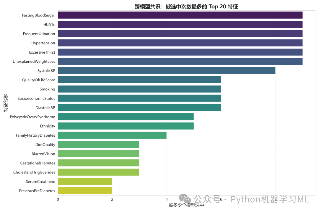
Pipeline,准确地找出最终被模型使用的特征。- 特征共识分析
代码统计了在所有单模型中,每个特征被选中的次数。如果一个特征被多个高性能模型同时选中,这强烈暗示了它是一个对预测目标至关重要的“强特征”。
- 可视化
通过条形图展示了被选中次数最多的特征。这个图非常有价值,它为我们提供了超越单个模型重要性排序的、更具鲁棒性的“特征共识”,帮助我们理解问题的核心驱动因素。
python
# ==================== 第十七部分:特征重要性解析 ====================
print("\n" + "=" * 70)
print("🔍 第十七部分:模型特征使用情况解析")
print("=" * 70)


defextract_features_from_pipeline(pipeline, original_features):
"""从Pipeline中提取最终使用的特征名"""
    current_features = np.array(original_features)

    step_names = pipeline.named_steps.keys()

if'selector'in step_names:
        selector = pipeline.named_steps['selector']
try:
            mask = selector.get_support()
            current_features = current_features[mask]
except:
pass

if'poly'in step_names:
        poly = pipeline.named_steps['poly']
try:
ifhasattr(poly, 'get_feature_names_out'):
                current_features = poly.get_feature_names_out(current_features)
else:
                current_features = poly.get_feature_names(current_features)
except:
pass

return current_features


feature_analysis_results = {}
all_selected_features = []

print("\n📂 正在解析各模型使用的特征...\n")

for model_name, pipeline in optimized_models.items():
if'Ensemble'in model_name:
continue

print(f"📌 [{model_name}]")

    final_feats = extract_features_from_pipeline(pipeline, feature_names)
    feature_analysis_results[model_name] = final_feats
    all_selected_features.extend(final_feats)

    n_orig = len(feature_names)
    n_final = len(final_feats)
    ratio = (n_final / n_orig) * 100

print(f"   原始特征: {n_orig} → 最终特征: {n_final} (保留率 {ratio:.1f}%)")
print(f"   特征预览: {list(final_feats[:5])}{'...'if n_final > 5else''}")
print()

result_file = os.path.join(output_dir, 'final_selected_features_list.txt')
withopen(result_file, 'w', encoding='utf-8') as f:
    f.write("=" * 70 + "\n")
    f.write("各模型最终使用的特征列表\n")
    f.write("=" * 70 + "\n\n")
for m_name, feats in feature_analysis_results.items():
        f.write(f"模型: {m_name}\n")
        f.write(f"特征数量: {len(feats)}\n")
        f.write(f"特征列表: {', '.join(feats)}\n")
        f.write("-" * 70 + "\n")

print(f"✅ 特征列表已保存: {result_file}")

if all_selected_features:
    feat_counts = Counter(all_selected_features)
    common_feats = feat_counts.most_common(20)

if common_feats:
        names, counts = zip(*common_feats)

        plt.figure(figsize=(12, 8))
        sns.barplot(x=list(counts), y=list(names), palette='viridis')
        plt.title(f'跨模型共识:被选中次数最多的 Top {len(names)} 特征',
                  fontsize=14, fontweight='bold')
        plt.xlabel('被多少个模型选中', fontsize=12)
        plt.ylabel('特征名称', fontsize=12)
        plt.grid(axis='x', linestyle='--', alpha=0.5)
        plt.tight_layout()
        plt.savefig(os.path.join(output_dir, '13_common_important_features.png'), dpi=300)
        plt.show()
print(f"✅ 特征共识图已保存: {output_dir}/13_common_important_features.png")
阶段 18: 保存模型信息
这是整个流程的最后一步,负责将所有重要的产出物保存到磁盘,以便未来部署、复现或分享。
作用解释:
best_model.pkl保存最终性能排行榜上第一名的模型。这个文件可以直接被加载到生产环境中,对新的数据进行预测。
all_optimized_models.pkl保存所有优化过的模型,以备将来可能需要使用其他模型或进行进一步分析。
best_parameters.json将所有模型的最佳超参数组合以及它们在预处理流程中的最佳选择(如用哪种缩放、采样、特征选择方法)保存为易于阅读的JSON文件。这对于记录实验配置、撰写报告和复现结果至关重要。
这一步标志着从实验研究到生产部署的关键过渡,确保了分析成果的实用性和可追溯性。
python
#显示中文负号
plt.rcParams['font.sans-serif'] = ['microsoft YaHei']  # 用黑体显示中文
plt.rcParams['axes.unicode_minus'] = False# 用来正常显示负号
# ==================== 第十八部分:保存最佳模型 ====================
print("\n" + "=" * 70)
print("💾 第十八部分:保存最佳模型")
print("=" * 70)

best_model_name = results_df.iloc[0]['Model']
best_model = optimized_models[best_model_name]
best_auc = results_df.iloc[0]['ROC-AUC']

print(f"\n🏆 最佳模型: {best_model_name} (AUC={best_auc:.4f})")

model_file = os.path.join(output_dir, 'best_model.pkl')
joblib.dump(best_model, model_file)
print(f"✅ 最佳模型已保存: {model_file}")

all_models_file = os.path.join(output_dir, 'all_optimized_models.pkl')
joblib.dump(optimized_models, all_models_file)
print(f"✅ 所有模型已保存: {all_models_file}")

params_file = os.path.join(output_dir, 'best_parameters.json')
withopen(params_file, 'w', encoding='utf-8') as f:
    serializable_params = {}
for model_name, params in best_params_dict.items():
        serializable_params[model_name] = {
            k: (v.item() ifisinstance(v, np.generic) else v)
for k, v in params.items()
        }
    json.dump(serializable_params, f, indent=2, ensure_ascii=False)
print(f"✅ 最佳参数已保存: {params_file}")
阶段 19: 增强型混淆矩阵与临床指标分析
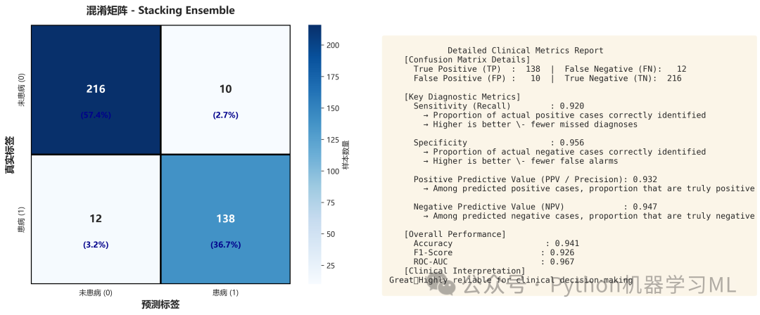
此阶段超越了标准的混淆矩阵,为模型的评估引入了多个关键的临床诊断指标,并提供了直观的解释和对比。
作用解释:
plot_enhanced_confusion_matrix这个函数是核心。它生成一个双面板图:
- 灵敏度 (Sensitivity / Recall)
模型正确识别出所有真正患病者的能力。高灵敏度意味着漏诊率低。
- 特异度 (Specificity)
模型正确识别出所有健康者的能力。高特异度意味着误诊率低。
- 阳性预测值 (PPV / Precision)
当模型预测为“患病”时,该预测正确的概率。
- 阴性预测值 (NPV)
当模型预测为“未患病”时,该预测正确的概率。
- 左侧 (混淆矩阵)
一个美化过的混淆矩阵,不仅显示了预测正确的样本数(TP, TN)和错误的样本数(FP, FN),还标注了它们在总样本中的百分比。
- 右侧 (临床报告)
一个详细的文本报告,解释并计算了几个在医学诊断中至关重要的指标:
- 灵敏度 (Sensitivity / Recall)
- 临床解读
函数包含了一个
get_clinical_interpretation的逻辑,根据灵敏度和特异度给出一个简单的英文定性评价(如 "Great"、"Good"),这使得非技术人员也能快速理解模型的可靠性。 - 雷达图对比
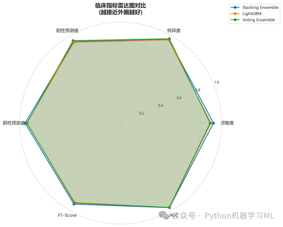
为了直观比较Top 3模型的临床综合性能,代码绘制了一个雷达图。每个顶点代表一个关键临床指标,模型的线条所包围的面积越大、形状越饱满,说明其综合临床表现越好。
这一整套分析使得模型评估不再仅仅停留在AUC等宏观指标上,而是深入到了模型的临床实用性层面。
python
# ==================== 补充导入必要的库 ====================
from sklearn.calibration import calibration_curve
from sklearn.inspection import permutation_importance
import json
from datetime import datetime
import sys
from collections import Counter

#  第十九部分:增强型混淆矩阵与临床指标 ====================
print("\n" + "=" * 70)
print("🔲 第十九部分:增强型混淆矩阵与临床指标")
print("=" * 70)


defplot_enhanced_confusion_matrix(y_true, y_pred, y_proba, model_name, save_path):
"""绘制增强型混淆矩阵,包含多个临床指标"""
    cm = confusion_matrix(y_true, y_pred)
    tn, fp, fn, tp = cm.ravel()

    sensitivity = tp / (tp + fn) if (tp + fn) > 0else0
    specificity = tn / (tn + fp) if (tn + fp) > 0else0
    ppv = tp / (tp + fp) if (tp + fp) > 0else0
    npv = tn / (tn + fn) if (tn + fn) > 0else0
    accuracy = (tp + tn) / (tp + tn + fp + fn)
    f1 = 2 * tp / (2 * tp + fp + fn) if (2 * tp + fp + fn) > 0else0
    auc = roc_auc_score(y_true, y_proba)

defget_clinical_interpretation(sens, spec):
if sens >= 0.9and spec >= 0.9:
#英文
return" Great:Highly reliable for clinical decision-making"
elif sens >= 0.8and spec >= 0.8:
return" Good:Very reliable for clinical decision-making"
elif sens >= 0.7or spec >= 0.7:
return" Moderate:Reliable for clinical decision-making"
else:
return"Poor:Not reliable for clinical decision-making"

    fig, axes = plt.subplots(1, 2, figsize=(16, 6))

    ax1 = axes[0]
    sns.heatmap(cm, annot=True, fmt='d', cmap='Blues', ax=ax1,
                xticklabels=['未患病 (0)', '患病 (1)'],
                yticklabels=['未患病 (0)', '患病 (1)'],
                cbar_kws={'label': '样本数量'}, square=True,
                linewidths=2, linecolor='black',
                annot_kws={'size': 14, 'weight': 'bold'})

    total = np.sum(cm)
for i inrange(2):
for j inrange(2):
            percentage = cm[i, j] / total * 100
            ax1.text(j + 0.5, i + 0.7, f'({percentage:.1f}%)',
                     ha='center', va='center', fontsize=11,
                     color='darkblue', fontweight='bold')

    ax1.set_xlabel('预测标签', fontsize=13, fontweight='bold')
    ax1.set_ylabel('真实标签', fontsize=13, fontweight='bold')
    ax1.set_title(f'混淆矩阵 - {model_name}', fontsize=14, fontweight='bold', pad=15)

    ax2 = axes[1]
    ax2.axis('off')
    metrics_text = f"""
             Detailed Clinical Metrics Report
    [Confusion Matrix Details]
      True Positive (TP)  : {tp:4d}  |  False Negative (FN): {fn:4d}
      False Positive (FP) : {fp:4d}  |  True Negative (TN): {tn:4d}

    [Key Diagnostic Metrics]
      Sensitivity (Recall)        : {sensitivity:.3f}
        → Proportion of actual positive cases correctly identified
        → Higher is better \- fewer missed diagnoses

      Specificity                 : {specificity:.3f}
        → Proportion of actual negative cases correctly identified
        → Higher is better \- fewer false alarms

      Positive Predictive Value (PPV / Precision): {ppv:.3f}
        → Among predicted positive cases, proportion that are truly positive

      Negative Predictive Value (NPV)            : {npv:.3f}
        → Among predicted negative cases, proportion that are truly negative

    [Overall Performance]
      Accuracy                   : {accuracy:.3f}
      F1-Score                  : {f1:.3f}
      ROC-AUC                   : {auc:.3f}
    [Clinical Interpretation]
{get_clinical_interpretation(sensitivity, specificity)}
    """

    ax2.text(0.05, 0.95, metrics_text, transform=ax2.transAxes,
             fontsize=11, verticalalignment='top', fontfamily='monospace',
             bbox=dict(boxstyle='round', facecolor='wheat', alpha=0.3))

    plt.tight_layout()
    plt.savefig(save_path, dpi=300, bbox_inches='tight')
    plt.show()

return {
'sensitivity': sensitivity,
'specificity': specificity,
'ppv': ppv,
'npv': npv,
'accuracy': accuracy,
'f1': f1,
'auc': auc
    }


print("\n🔍 生成Top 3模型的详细混淆矩阵分析...\n")
top3_models = results_df.head(3)
clinical_metrics_summary = []

for idx, row in top3_models.iterrows():
    model_name = row['Model']
print("=" * 60)
print(f"分析模型: {model_name}")
print("=" * 60)

    y_pred = all_predictions[model_name]['y_pred']
    y_proba = all_predictions[model_name]['y_pred_proba']

    save_path = f'{output_dir}/14_confusion_matrix_{model_name.replace(" ", "_")}.png'
    metrics = plot_enhanced_confusion_matrix(y_test, y_pred, y_proba,
                                             model_name, save_path)

    metrics['Model'] = model_name
    clinical_metrics_summary.append(metrics)
print(f"✅ 已保存: {save_path}\n")

clinical_df = pd.DataFrame(clinical_metrics_summary)
clinical_df.to_csv(f'{output_dir}/clinical_metrics_comparison.csv', index=False)
print(f"✅ 临床指标对比已保存: {output_dir}/clinical_metrics_comparison.csv")

print("\n📊 生成临床指标雷达图对比...")
fig, ax = plt.subplots(figsize=(10, 10), subplot_kw=dict(projection='polar'))

metrics_list = ['sensitivity', 'specificity', 'ppv', 'npv', 'f1', 'auc']
metrics_labels = ['灵敏度', '特异度', '阳性预测值', '阴性预测值', 'F1-Score', 'AUC']

angles = np.linspace(0, 2 * np.pi, len(metrics_list), endpoint=False).tolist()
angles += angles[:1]

colors = ['#1f77b4', '#ff7f0e', '#2ca02c']
for i, metrics_dict inenumerate(clinical_metrics_summary):
    values = [metrics_dict[m] for m in metrics_list]
    values += values[:1]

    ax.plot(angles, values, 'o-', linewidth=2, label=metrics_dict['Model'], color=colors[i])
    ax.fill(angles, values, alpha=0.15, color=colors[i])

ax.set_xticks(angles[:-1])
ax.set_xticklabels(metrics_labels, fontsize=11)
ax.set_ylim(0, 1)
ax.set_yticks([0.2, 0.4, 0.6, 0.8, 1.0])
ax.set_yticklabels(['0.2', '0.4', '0.6', '0.8', '1.0'], fontsize=9)
ax.grid(True, linestyle='--', alpha=0.5)
ax.set_title('临床指标雷达图对比\n(越接近外圈越好)',
             fontsize=14, fontweight='bold', pad=20)
ax.legend(loc='upper right', bbox_to_anchor=(1.3, 1.1), fontsize=10)

plt.tight_layout()
plt.savefig(f'{output_dir}/14_clinical_metrics_radar.png', dpi=300, bbox_inches='tight')
plt.show()
print(f"✅ 雷达图已保存: {output_dir}/14_clinical_metrics_radar.png")
阶段 20: 模型校准曲线分析
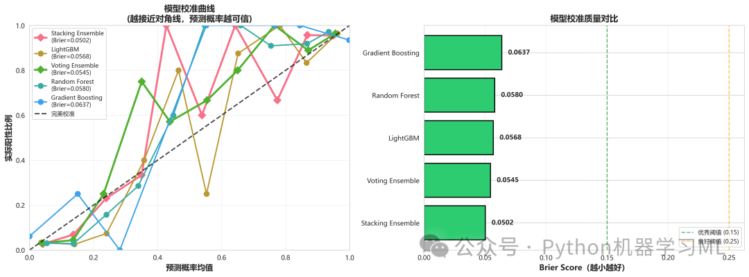
这个阶段用于评估模型预测概率的可信度。一个好的模型不仅要能正确分类,其输出的概率值也应该能真实反映事件发生的可能性。
作用解释:
- 核心问题
如果模型预测一个病人有80%的概率患病,我们能否相信这个“80%”是准确的?
- 校准曲线
- 横轴
模型预测的概率(例如,所有被预测为80%概率的样本)。
- 纵轴
这些样本中实际患病的比例。
- 理想情况
曲线应该紧贴对角线(y=x)。这意味着当模型预测概率为X%时,这些样本中实际患病的比例也确实是X%。
- 横轴
- Brier Score
-
它是衡量校准度的单一数值指标,本质是预测概率与真实结果(0或1)之间均方误差。
- Brier Score越低,说明模型的预测概率越准确、越值得信赖
-
- 可视化解读
- 左图 (校准曲线)
直观展示了每个模型偏离“完美校准”(对角线)的程度。
- 右图 (Brier Score对比)
通过条形图快速比较各个模型的校准质量,得分越低越好。
- 左图 (校准曲线)
此分析对于需要根据具体风险概率来制定不同干预措施的场景(例如,风险>70%立即手术,风险40-70%进一步检查)至关重要。
python
# ==== 第二十部分:模型校准曲线分析 ====================
print("\n" + "=" * 70)
print("📏 第二十部分:模型校准曲线分析")
print("=" * 70)


defplot_calibration_curves(models_dict, y_test, save_path):
"""绘制多个模型的校准曲线"""
    fig, axes = plt.subplots(1, 2, figsize=(16, 6))

    ax1 = axes[0]
    brier_scores = {}

for model_name, pred_data in models_dict.items():
        y_proba = pred_data['y_pred_proba']

        fraction_of_positives, mean_predicted_value = calibration_curve(
            y_test, y_proba, n_bins=10, strategy='uniform'
        )

        brier_score = np.mean((y_proba - y_test) ** 2)
        brier_scores[model_name] = brier_score

        linewidth = 3if'Ensemble'in model_name else2
        marker = 'D'if'Ensemble'in model_name else'o'
        ax1.plot(mean_predicted_value, fraction_of_positives,
                 marker=marker, linewidth=linewidth, markersize=8,
                 label=f'{model_name}\n(Brier={brier_score:.4f})')

    ax1.plot([0, 1], [0, 1], 'k--', linewidth=2, label='完美校准', alpha=0.7)

    ax1.set_xlabel('预测概率均值', fontsize=12, fontweight='bold')
    ax1.set_ylabel('实际阳性比例', fontsize=12, fontweight='bold')
    ax1.set_title('模型校准曲线\n(越接近对角线,预测概率越可信)', fontsize=13, fontweight='bold')
    ax1.legend(loc='upper left', fontsize=9)
    ax1.grid(True, alpha=0.3)
    ax1.set_xlim([0, 1])
    ax1.set_ylim([0, 1])

    ax2 = axes[1]
    brier_df = pd.DataFrame(list(brier_scores.items()),
                            columns=['Model', 'Brier Score'])
    brier_df = brier_df.sort_values('Brier Score')

    colors = ['#2ecc71'if x < 0.15else ('#f39c12'if x < 0.25else'#e74c3c')
for x in brier_df['Brier Score']]

    ax2.barh(brier_df['Model'], brier_df['Brier Score'], color=colors,
             edgecolor='black', linewidth=1.5)
    ax2.set_xlabel('Brier Score(越小越好)', fontsize=12, fontweight='bold')
    ax2.set_title('模型校准质量对比', fontsize=13, fontweight='bold')

    ax2.axvline(x=0.15, color='green', linestyle='--', linewidth=1.5,
                alpha=0.6, label='优秀阈值 (0.15)')
    ax2.axvline(x=0.25, color='orange', linestyle='--', linewidth=1.5,
                alpha=0.6, label='良好阈值 (0.25)')
    ax2.legend(loc='lower right', fontsize=9)
    ax2.grid(axis='x', alpha=0.3)

for i, v inenumerate(brier_df['Brier Score']):
        ax2.text(v + 0.005, i, f'{v:.4f}', va='center', fontsize=10, fontweight='bold')

    plt.tight_layout()
    plt.savefig(save_path, dpi=300, bbox_inches='tight')
    plt.show()

return brier_df


print("\n📊 生成校准曲线...\n")
top5_for_calibration = {name: all_predictions[name]
for name in results_df.head(5)['Model']}

brier_results = plot_calibration_curves(
    top5_for_calibration, y_test,
f'{output_dir}/15_calibration_curves.png'
)

print("\n📋 Brier Score 结果解读:")
print(brier_results.to_string(index=False))
print("\n💡 Brier Score 评级标准:")
print("  • < 0.10: 极好  ⭐⭐⭐⭐⭐")
print("  • 0.10-0.15: 优秀  ⭐⭐⭐⭐")
print("  • 0.15-0.25: 良好  ⭐⭐⭐")
print("  • > 0.25: 需改进  ⭐⭐")

brier_results.to_csv(f'{output_dir}/brier_scores.csv', index=False)
print(f"\n✅ 校准曲线已保存: {output_dir}/15_calibration_curves.png")
print(f"✅ Brier Score已保存: {output_dir}/brier_scores.csv")
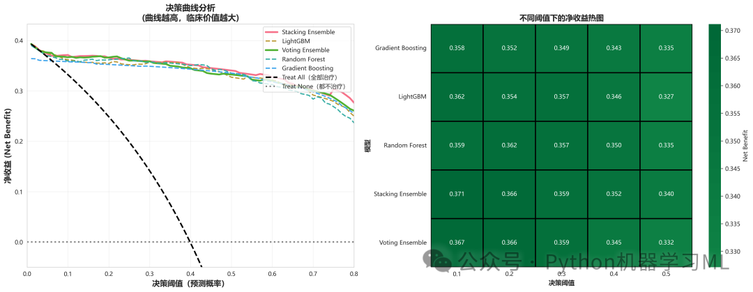
阶段 21: 决策曲线分析 (DCA)
这是目前最前沿、最能体现模型临床实用价值的评估方法。它帮助决策者(如医生)判断,在不同的风险阈值下,使用这个模型辅助决策是否比传统的“一刀切”(全部治疗或全部不治疗)策略更好。
作用解释:
- 核心概念 (净收益 Net Benefit)
DCA的核心是计算“净收益”。它量化了使用模型带来的好处(正确识别并治疗了患者)减去带来的坏处(错误地给健康人进行了不必要的干预)后的净效果。
- 决策曲线图解读
- 横轴 (决策阈值)
医生/患者愿意接受干预的最低风险概率。例如,阈值为20%意味着“如果患病风险超过20%,我就采取行动”。
- 纵轴 (净收益)
在该决策阈值下,使用模型带来的净收益。
- 三条关键线
- 判断标准
在某个决策阈值范围内,如果一个模型的曲线高于“Treat All”和“Treat None”这两条线,就说明在这个范围内使用该模型是有临床价值的。曲线越高,价值越大。
- 模型曲线
代表使用该模型进行决策的净收益。
- "Treat All"线 (全部治疗)
代表不使用模型,直接对所有人进行干预的策略。
- "Treat None"线 (都不治疗)
净收益恒为0的水平线,代表不采取任何干预。
- 横轴 (决策阈值)
- 热图与最优阈值
- 右侧热图
直观展示了在几个关键阈值(如10%, 20%...)下,不同模型的净收益对比。
- 最优阈值计算
代码还自动找出了每个模型能达到最大净收益时所对应的“最优决策阈值”,为临床实践提供了直接的、数据驱动的建议。
- 右侧热图
DCA将模型评估从一个纯粹的统计问题,转化为了一个与实际决策紧密结合的效用问题,是衡量预测模型临床转化潜力的金标准。
python
#  第二十一部分:决策曲线分析(DCA)====================
print("\n" + "=" * 70)
print("📊 第二十一部分:决策曲线分析(Decision Curve Analysis)")
print("=" * 70)


defcalculate_net_benefit(y_true, y_proba, threshold):
"""计算指定阈值下的净收益"""
    y_pred = (y_proba >= threshold).astype(int)

iflen(np.unique(y_pred)) == 1:
if y_pred[0] == 1:
            tp = np.sum(y_true == 1)
            fp = np.sum(y_true == 0)
            tn = fn = 0
else:
            tn = np.sum(y_true == 0)
            fn = np.sum(y_true == 1)
            tp = fp = 0
else:
        tn, fp, fn, tp = confusion_matrix(y_true, y_pred).ravel()

    n = len(y_true)
if threshold >= 1.0:
return0.0

    net_benefit = (tp / n) - (fp / n) * (threshold / (1 - threshold))
return net_benefit


defplot_decision_curve(models_dict, y_test, save_path):
"""绘制决策曲线"""
    fig, axes = plt.subplots(1, 2, figsize=(18, 7))
    thresholds = np.arange(0.01, 0.99, 0.01)

    ax1 = axes[0]
    model_nb_data = {}

for model_name, pred_data in models_dict.items():
        y_proba = pred_data['y_pred_proba']
        net_benefits = [calculate_net_benefit(y_test, y_proba, t) for t in thresholds]
        model_nb_data[model_name] = net_benefits

        linewidth = 3if'Ensemble'in model_name else2
        linestyle = '-'if'Ensemble'in model_name else'--'
        ax1.plot(thresholds, net_benefits, linewidth=linewidth,
                 linestyle=linestyle, label=model_name)

    prevalence = np.mean(y_test)
    treat_all = []
for t in thresholds:
if t >= 1.0:
            treat_all.append(0.0)
else:
            treat_all.append(prevalence - (1 - prevalence) * (t / (1 - t)))
    ax1.plot(thresholds, treat_all, 'k--', linewidth=2.5, label='Treat All(全部治疗)')
    ax1.axhline(y=0, color='gray', linestyle=':', linewidth=2.5, label='Treat None(都不治疗)')

    ax1.set_xlabel('决策阈值(预测概率)', fontsize=13, fontweight='bold')
    ax1.set_ylabel('净收益 (Net Benefit)', fontsize=13, fontweight='bold')
    ax1.set_title('决策曲线分析\n(曲线越高,临床价值越大)', fontsize=14, fontweight='bold')
    ax1.legend(loc='upper right', fontsize=10)
    ax1.grid(True, alpha=0.3)
    ax1.set_xlim([0, 0.8])

    all_nb = []
for nb in model_nb_data.values():
        all_nb.extend(nb[:80])
    all_nb.extend(treat_all[:80])
    y_max = max(all_nb) * 1.1if all_nb else0.5
    ax1.set_ylim([-0.05, y_max])

    ax2 = axes[1]
    key_thresholds = [0.1, 0.2, 0.3, 0.4, 0.5]
    comparison_data = []

for model_name, nb_values in model_nb_data.items():
for thresh in key_thresholds:
            idx = int(thresh * 100) - 1
if idx < len(nb_values):
                comparison_data.append({
'Model': model_name,
'Threshold': thresh,
'Net Benefit': nb_values[idx]
                })

    comp_df = pd.DataFrame(comparison_data)
    pivot_df = comp_df.pivot(index='Model', columns='Threshold', values='Net Benefit')

    sns.heatmap(pivot_df, annot=True, fmt='.3f', cmap='RdYlGn',
                center=0, ax=ax2, cbar_kws={'label': 'Net Benefit'},
                linewidths=1.5, linecolor='black', annot_kws={'size': 10})
    ax2.set_title('不同阈值下的净收益热图', fontsize=13, fontweight='bold')
    ax2.set_xlabel('决策阈值', fontsize=11, fontweight='bold')
    ax2.set_ylabel('模型', fontsize=11, fontweight='bold')

    plt.tight_layout()
    plt.savefig(save_path, dpi=300, bbox_inches='tight')
    plt.show()

print("\n🎯 各模型推荐的最优决策阈值:")
    optimal_thresholds = []
for model_name, nb_values in model_nb_data.items():
        search_range = nb_values[10:70]
if search_range:
            optimal_idx = np.argmax(search_range) + 10
            optimal_thresh = thresholds[optimal_idx]
            optimal_nb = nb_values[optimal_idx]
            optimal_thresholds.append({
'Model': model_name,
'Optimal_Threshold': optimal_thresh,
'Max_Net_Benefit': optimal_nb
            })
print(f"  {model_name:30s}: 阈值={optimal_thresh:.2f}, 净收益={optimal_nb:.4f}")

return comp_df, pd.DataFrame(optimal_thresholds)


print("\n⏳ 正在计算决策曲线...\n")
top5_for_dca = {name: all_predictions[name] for name in results_df.head(5)['Model']}

dca_comparison, optimal_thresh_df = plot_decision_curve(
    top5_for_dca, y_test, f'{output_dir}/16_decision_curve_analysis.png'
)

dca_comparison.to_csv(f'{output_dir}/decision_curve_data.csv', index=False)
optimal_thresh_df.to_csv(f'{output_dir}/optimal_thresholds.csv', index=False)
print(f"\n✅ 决策曲线已保存: {output_dir}/16_decision_curve_analysis.png")
print(f"✅ DCA数据已保存: {output_dir}/decision_curve_data.csv")
print(f"✅ 最优阈值已保存: {output_dir}/optimal_thresholds.csv")

print("\n💡 决策曲线解读:")
print("  1. 净收益 > 0: 模型优于'不治疗'策略")
print("  2. 净收益 > Treat All线: 模型优于'全部治疗'策略")
print("  3. 阈值选择应根据临床成本和风险权衡")
print("  4. 对于筛查,通常选择较低阈值(0.1-0.3)以提高灵敏度")
print("  5. 对于确诊,可选择较高阈值(0.4-0.6)以提高特异度")
阶段 22: SHAP 分析准备与计算 (针对 Stacking 模型)
这个阶段是整个 SHAP 分析的核心准备和计算部分。由于 Stacking 模型是一个“黑箱”中的“黑箱”(它由多个其他模型组成),不能使用为树模型优化的 TreeExplainer。因此,这里必须使用更通用但计算更慢的 KernelExplainer。
作用解释:
- 加载模型与数据
首先,代码加载之前训练并保存的最佳模型(Stacking Ensemble)和对应的特征名。
- 准备输入数据
SHAP 计算可能非常耗时,特别是
KernelExplainer。为了在合理的时间内得到结果,代码从全量数据中随机抽取一部分样本(MAX_SHAP_SAMPLES = 150)用于计算,值越大消耗时间越多,前期可设置较小值,快速验证。 - 创建解释器 (Explainer)
这是关键一步。代码创建了一个
shap.KernelExplainer。它通过向模型输入不同的特征组合来“探测”模型的行为,从而估算每个特征的贡献。为了加速,它没有使用所有训练数据作为背景,而是使用shap.kmeans将背景数据聚类成20个“代表点”,这大大减少了计算量。可自行根据情况更改。 - 计算 SHAP 值
代码调用
explainer.shap_values()来执行核心计算。对于二分类问题,KernelExplainer会返回一个包含两个数组的列表(分别对应类别0和类别1的SHAP值)。代码正确地提取了我们关心的正类(类别1)的 SHAP 值用于后续分析。
python
# =第二十四部分:SHAP 特征重要性可视化 ====================
print("\n" + "=" * 70)
print("🔍 第二十四部分:SHAP 特征重要性分析")
print("=" * 70)

import shap
import joblib
import matplotlib.pyplot as plt
import numpy as np
import pandas as pd

# 设置中文字体,防止乱码
plt.rcParams['font.sans-serif'] = ['microsoft YaHei']
plt.rcParams['axes.unicode_minus'] = False# 用来正常显示负号

# 1. 加载已保存的最佳模型和特征信息
best_model_path = r'saved_models_diabetes\best_model_Stacking_Ensemble.pkl'
feature_info_path = r'saved_models_diabetes\feature_info.pkl'

print(f"\n⏳ 正在加载最佳模型: {best_model_path}")
loaded_model = joblib.load(best_model_path)

print(f"⏳ 正在加载特征信息: {feature_info_path}")
loaded_feature_info = joblib.load(feature_info_path)

feature_names_for_shap = loaded_feature_info['feature_names']
print(f"✅ 加载完成,特征数: {len(feature_names_for_shap)}")

# 2. 准备用于 SHAP 的特征数据
print("\n📊 准备 SHAP 输入数据...")
# 确保数据只包含模型训练时的特征
X_for_shap = data_clean[feature_names_for_shap].copy()

# 为了计算速度(KernelExplainer 很慢),这里限制样本数量
# 建议设置在 50-100 之间,太少会导致画图为空,太多计算会非常慢
MAX_SHAP_SAMPLES = 150
iflen(X_for_shap) > MAX_SHAP_SAMPLES:
    X_sample = X_for_shap.sample(n=MAX_SHAP_SAMPLES, random_state=42)
else:
    X_sample = X_for_shap

print(f"  • SHAP 计算样本数: {len(X_sample)}")

# 3. 创建 SHAP Explainer (针对 Stacking 模型使用 KernelExplainer)
print("\n🧠 正在创建 SHAP 解释器...")

# Stacking 模型通常不支持 TreeExplainer,必须使用 KernelExplainer
# 为了加速 KernelExplainer,我们需要对背景数据进行摘要(K-Means 聚类)
# 使用约 20-50 个中心点来代表背景分布
background_data_summary = shap.kmeans(X_for_shap, 20)

try:
# 使用 predict_proba 确保输出概率
    explainer = shap.KernelExplainer(loaded_model.predict_proba, background_data_summary)
print("✅ 成功创建 KernelExplainer (适用于 Stacking 模型)")
except Exception as e:
print(f"⚠️ 创建 Explainer 出现警告,尝试使用原始样本作为背景: {e}")
    explainer = shap.KernelExplainer(loaded_model.predict_proba, X_sample)

# 4. 计算 SHAP 值
print("\n⏳ 正在计算 SHAP 值(这可能需要几分钟,请耐心等待)...")
try:
# 计算 SHAP 值
    shap_values_raw = explainer.shap_values(X_sample)

# 处理 SHAP 返回值格式
# 对于二分类,KernelExplainer 通常返回一个 list,包含两个数组 [class0_shap, class1_shap]
ifisinstance(shap_values_raw, list):
print(f"  • 检测到分类模型输出 (List 长度: {len(shap_values_raw)}),提取正类(Class 1) SHAP 值")
        shap_values_for_plot = shap_values_raw[1]
else:
# 如果是回归或特殊情况,直接使用
        shap_values_for_plot = shap_values_raw

# 再次确认维度是 (n_samples, n_features)
iflen(shap_values_for_plot.shape) == 3:
# 如果意外出现了交互值维度,尝试降维或报错
print("⚠️ 警告:检测到 3D SHAP 值,尝试取平均或修正...")
        shap_values_for_plot = shap_values_for_plot[:, :, 0]  # 仅作示例,通常 KernelExplainer 不会返回 3D

print(f"✅ SHAP 值计算完成,数据形状: {shap_values_for_plot.shape}")

except Exception as e:
print(f"❌ 计算 SHAP 值失败: {e}")
    shap_values_for_plot = None
阶段 23: 标准 SHAP 可视化
在成功计算出 SHAP 值后,这个阶段生成了一系列标准的、信息丰富的 SHAP 可视化图表,用于从不同角度理解模型。
作用解释:
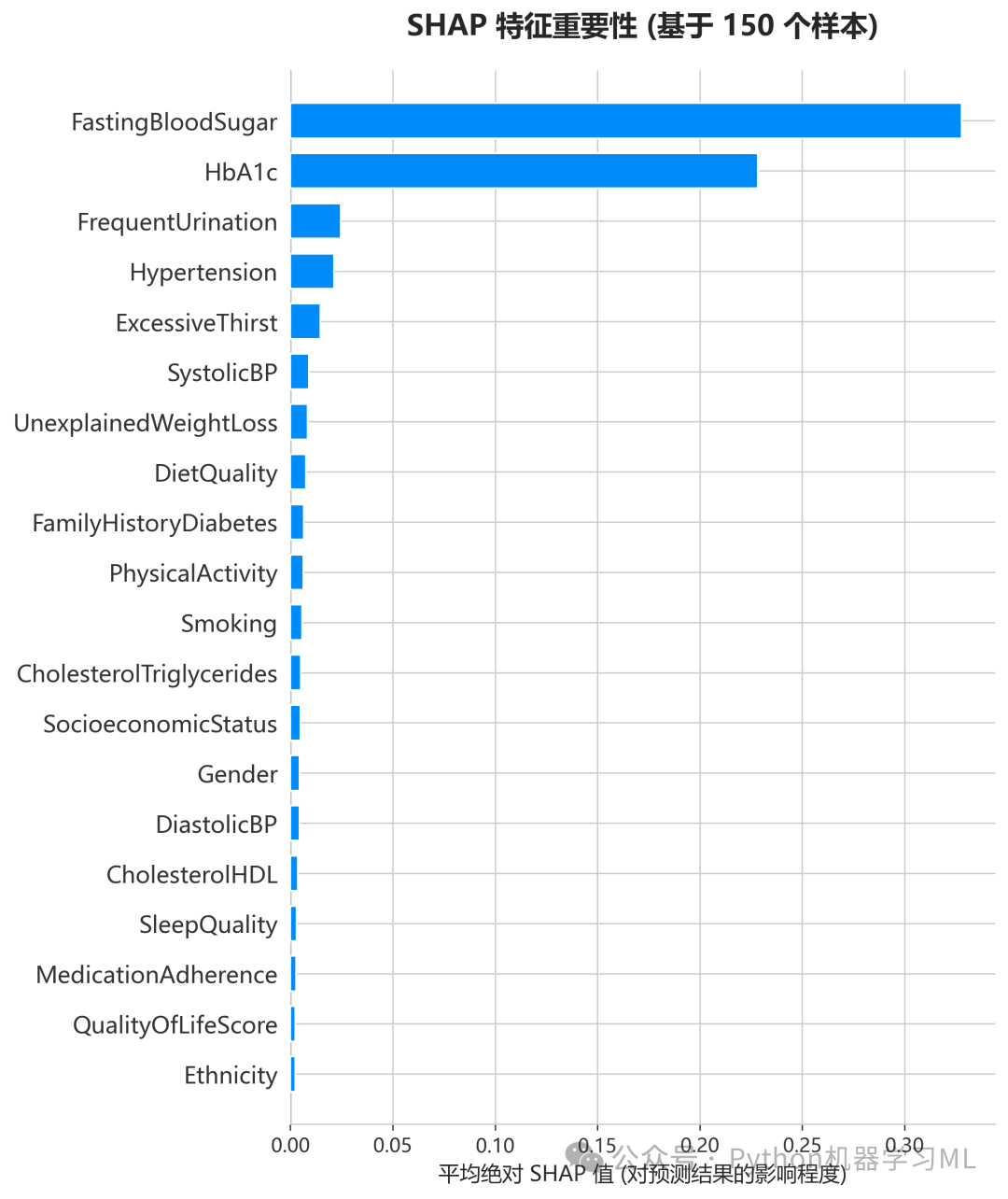
- 特征重要性条形图 (Bar Plot)
这是最直观的全局解释。它计算每个特征SHAP值的平均绝对值,然后按此值对特征进行排序。条形越长,代表该特征对模型的预测结果平均贡献越大,即越重要。
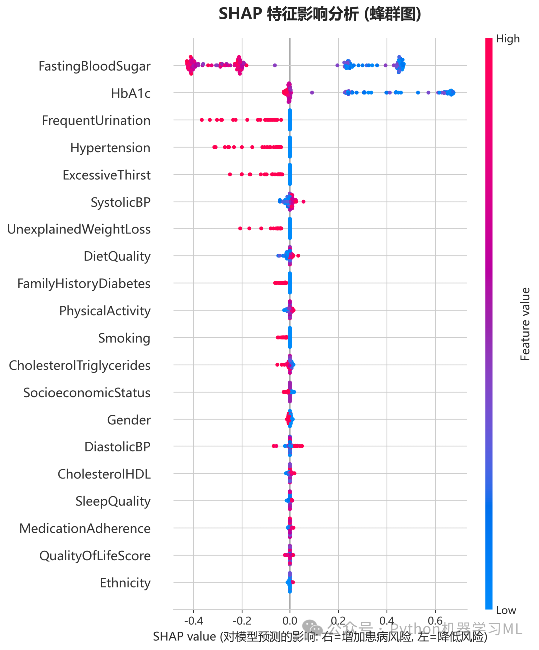
- 蜂群图 (Beeswarm Plot)
这是信息量最大的图之一。
-
每一行代表一个特征。
-
每一个点代表一个样本。
-
点的横轴位置是该样本在该特征上的 SHAP 值。正值表示该特征将预测推向“患病”,负值则推向“健康”。
-
点的颜色代表该特征自身的数值大小(红色=高值,蓝色=低值)。
-
通过此图,我们不仅能看到哪个特征重要,还能看到特征值的高低是如何影响预测方向的。例如,如果“葡萄糖”特征的红点(高血糖值)普遍在X轴右侧,说明高血糖会增加模型预测的患病风险。
-
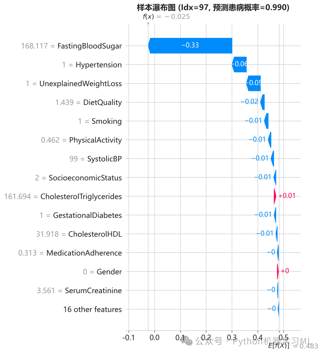
- 瀑布图 (Waterfall Plot)
此图用于解释单个样本的预测过程。它从模型的基准值(所有样本的平均预测概率)开始,像瀑布一样逐个展示每个特征是如何将预测值向上(红色)或向下(蓝色)推动,最终达到该样本的最终预测概率。这对于个案分析和解释具体某个病人的预测结果非常有用。
- 依赖图 (Dependence Plot)
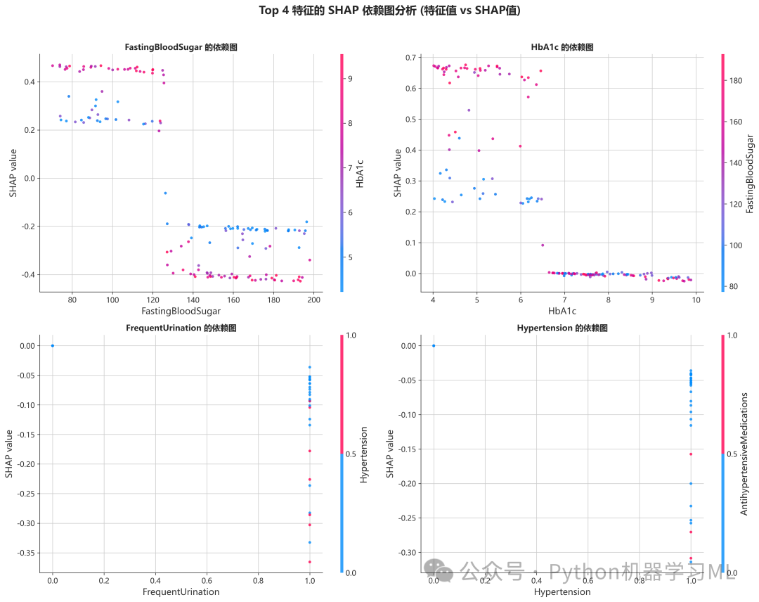
此图深入分析单个特征。它将某个特征的实际数值作为横轴,其对应的SHAP值作为纵轴。这揭示了特征值与模型贡献之间的非线性关系。图中的点还会根据与之交互最强的另一个特征进行着色,帮助我们发现特征间的交互效应。
python
# 5. 生成 SHAP 特征重要性条形图
if shap_values_for_plot isnotNone:
print("\n📈 正在绘制 SHAP 特征重要性条形图...")

    shap_output_path = f'{output_dir}/17_shap_feature_importance.png'

# 创建画布
    plt.figure(figsize=(12, 8))

# 绘制条形图 (Bar Plot)
# max_display 控制显示的特征数量,避免太拥挤
    shap.summary_plot(
        shap_values_for_plot,
        X_sample,
        feature_names=feature_names_for_shap,
        plot_type="bar",
        show=False,
        max_display=20
    )

# 调整布局和标题
    plt.title(f"SHAP 特征重要性 (基于 {MAX_SHAP_SAMPLES} 个样本)", fontsize=16, fontweight='bold', pad=20)
    plt.xlabel("平均绝对 SHAP 值 (对预测结果的影响程度)", fontsize=12)
    plt.tight_layout()

# 保存图片
    plt.savefig(shap_output_path, dpi=300, bbox_inches='tight')
    plt.show()
    plt.close()

print(f"✅ SHAP 特征重要性图已保存: {shap_output_path}")
else:
print("❌ 无法绘制 SHAP 图,因为 SHAP 值计算失败。")
#显示负号

# ==================== 接着上一步代码继续执行 ====================
# 确保 shap_values_for_plot 存在(即上一步计算成功)
if'shap_values_for_plot'inlocals() and shap_values_for_plot isnotNone:

# 转换 X_sample 为 numpy array 方便后续处理
    X_sample_array = X_sample.values

# ==================== 18. SHAP Summary Plot (蜂群图) ====================
print("\n📊 18. 生成 SHAP Summary Plot (蜂群图)...")

    shap_beeswarm_path = f'{output_dir}/18_shap_summary_beeswarm.png'

    plt.figure(figsize=(12, 10))
    shap.summary_plot(
        shap_values_for_plot,
        X_sample,  # 这里可以直接传 DataFrame,会自动显示列名
        feature_names=feature_names_for_shap,
        plot_type="dot",
        max_display=20,
        show=False
    )
    plt.title('SHAP 特征影响分析 (蜂群图)', fontsize=16, fontweight='bold', pad=20)
    plt.xlabel('SHAP value (对模型预测的影响: 右=增加患病风险, 左=降低风险)', fontsize=12)
    plt.tight_layout()
    plt.savefig(shap_beeswarm_path, dpi=300, bbox_inches='tight')
    plt.show()
    plt.close()
print(f"✅ SHAP 蜂群图已保存: {shap_beeswarm_path}")

# ==================== 19. 特征重要性数值统计 ====================
# 计算每个特征的平均绝对SHAP值
    shap_importance = np.abs(shap_values_for_plot).mean(0)

print(f"\n📊 特征重要性统计:")
print(f"  - 总特征数: {len(feature_names_for_shap)}")
print(f"  - 最高重要性值: {shap_importance.max():.4f}")
print(f"  - 平均重要性值: {shap_importance.mean():.4f}")

# 显示前10个最重要的特征
    top_10_idx = np.argsort(shap_importance)[-10:][::-1]
print(f"\n🏆 前10个最重要的特征 (基于 SHAP):")
for i, idx inenumerate(top_10_idx, 1):
print(f"  {i}. {feature_names_for_shap[idx]:<25}: {shap_importance[idx]:.4f}")

# ==================== 20. SHAP Waterfall Plot (瀑布图 - 单样本解释) ====================
print("\n📊 20. 生成 SHAP 瀑布图 (单样本详细解释)...")

# 1. 获取基准值 (Expected Value)
# KernelExplainer 的 expected_value 对于二分类通常是一个列表 [val0, val1]
    base_value = 0
ifisinstance(explainer.expected_value, (list, np.ndarray)):
# 取正类 (Class 1) 的基准值
        base_value = explainer.expected_value[1] iflen(explainer.expected_value) > 1else explainer.expected_value[0]
else:
        base_value = explainer.expected_value

print(f"ℹ️ 模型基准值 (Base Value/平均预测值): {base_value:.4f}")

# 2. 手动构建 Explanation 对象 (关键步骤:KernelExplainer 不直接返回此对象)
    shap_explanation_obj = shap.Explanation(
        values=shap_values_for_plot,
        base_values=base_value,
        data=X_sample_array,
        feature_names=feature_names_for_shap
    )

# 3. 选择一个具有代表性的样本(例如预测概率较高的样本)
# 计算样本的预测概率
    y_pred_proba_sample = loaded_model.predict_proba(X_sample)[:, 1]

# 找到预测概率最高的样本索引(或者你可以指定 sample_idx = 0)
    sample_idx = np.argmax(y_pred_proba_sample)

    shap_waterfall_path = f'{output_dir}/20_shap_waterfall_sample_{sample_idx}.png'

    plt.figure(figsize=(10, 8))
# 绘制瀑布图
    shap.plots.waterfall(
        shap_explanation_obj[sample_idx],
        max_display=15,
        show=False
    )
    plt.title(f'样本瀑布图 (Idx={sample_idx}, 预测患病概率={y_pred_proba_sample[sample_idx]:.3f})',
              fontsize=14, fontweight='bold')
    plt.tight_layout()
    plt.savefig(shap_waterfall_path, dpi=300, bbox_inches='tight')
    plt.show()
    plt.close()
print(f"✅ SHAP 瀑布图已保存: {shap_waterfall_path}")

# ==================== 21. SHAP Dependence Plot (依赖图) ====================
print("\n📊 21. 生成 SHAP 依赖图 (Top 4 特征)...")

    shap_dependence_path = f'{output_dir}/21_shap_dependence_top4.png'

# 选择前4个最重要的特征绘制依赖图
    top_4_features = np.argsort(shap_importance)[-4:][::-1]

    fig, axes = plt.subplots(2, 2, figsize=(16, 12))
    axes = axes.flatten()

for i, feat_idx inenumerate(top_4_features):
        feature_name = feature_names_for_shap[feat_idx]

        plt.sca(axes[i])
# interaction_index='auto' 会自动寻找与当前特征交互最强的特征进行着色
        shap.dependence_plot(
            feat_idx,
            shap_values_for_plot,
            X_sample,  # 传入 DataFrame 以显示正确轴标签
            feature_names=feature_names_for_shap,
            ax=axes[i],
            show=False,
            interaction_index='auto',
            alpha=0.8
        )
        axes[i].set_title(f'{feature_name} 的依赖图', fontsize=12, fontweight='bold')
        axes[i].set_ylabel('SHAP value')

    plt.suptitle('Top 4 特征的 SHAP 依赖图分析 (特征值 vs SHAP值)', fontsize=16, fontweight='bold', y=1.02)
    plt.tight_layout()
    plt.savefig(shap_dependence_path, dpi=300, bbox_inches='tight')
    plt.show()
    plt.close()
print(f"✅ SHAP 依赖图已保存: {shap_dependence_path}")

else:
print("❌ 跳过后续绘图步骤,因为 SHAP 值未成功计算。")
阶段 24: SHAP 深度统计与 Force Plot 可视化
这个阶段对 SHAP 值进行更深入的量化分析,并引入了另一种强大的可视化工具——Force Plot。
作用解释:
- SHAP 统计分析报告
代码将 SHAP 值转换为结构化的数据。它计算了每个特征的平均绝对影响(重要性)、SHAP值的标准差(波动性)、最大和最小影响,并将这些统计数据保存为 CSV 文件。这为撰写报告和进行定量分析提供了坚实的数据基础。
- 静态 Force Plot (力导图)
这与瀑布图类似,也是解释单个样本的预测。但它的展现形式更像一个“力平衡”图:
- 基准值 (Base Value)
是平衡点。
- 红色特征
是“推力”,将最终预测值向右(更高概率)推动。
- 蓝色特征
是“拉力”,将最终预测值向左(更低概率)拉动。
-
所有“力”的合力决定了最终的预测值
f(x)。这种图非常直观地展示了正负向贡献的特征及其贡献大小。
- 基准值 (Base Value)
- 交互式 Force Plot (HTML)
这是 Force Plot 的高级版本。它将所有样本的力导图堆叠起来,生成一个可以交互的 HTML 文件。在浏览器中打开它,你可以:
-
将鼠标悬停在任何位置,查看该特征对该样本的具体影响。
-
通过下拉菜单,按不同特征的值对所有样本进行排序,观察模式变化。
-
它会自动对相似的样本进行聚类,帮助发现具有相似决策逻辑的样本群体。
-
python
#  第二十五部分:SHAP 深度统计与可视化 ====================
print("\n" + "=" * 70)
print("🔍 第二十五部分:SHAP 深度统计与 Force Plot 可视化")
print("=" * 70)

import matplotlib.pyplot as plt
import pandas as pd
import numpy as np
import shap
import os

# 检查必要变量是否存在 (确保之前的 SHAP 计算已执行)
if'shap_values_for_plot'inlocals() and shap_values_for_plot isnotNone:

# --- 0. 准备基础数据 ---
# 确保 X_sample 是 DataFrame 格式
ifnotisinstance(X_sample, pd.DataFrame):
        X_sample_df = pd.DataFrame(X_sample, columns=feature_names_for_shap)
else:
        X_sample_df = X_sample.copy()

    X_sample_values = X_sample_df.values  # 用于绘图的数组格式

# 获取基准值 (Base Value / Expected Value)
# 为了保证模块独立性,这里重新获取一次基准值
    base_value = 0
ifhasattr(explainer, 'expected_value'):
ifisinstance(explainer.expected_value, (list, np.ndarray)):
# 二分类通常取 index 1 (正类)
            base_value = explainer.expected_value[1] iflen(explainer.expected_value) > 1else explainer.expected_value[
0]
else:
            base_value = explainer.expected_value

print(f"ℹ️ 当前模型基准值 (Base Value): {base_value:.4f}")

# ==================== 1. SHAP 值统计分析报告 ====================
print("\n📊 1. 生成 SHAP 统计分析报告...")

# 创建统计 DataFrame
    shap_stats_df = pd.DataFrame({
'Feature': feature_names_for_shap,
'Mean_|SHAP|': np.abs(shap_values_for_plot).mean(0),  # 平均绝对影响 (重要性)
'Std_SHAP': shap_values_for_plot.std(0),  # 波动性
'Max_|SHAP|': np.abs(shap_values_for_plot).max(0),  # 最大单次影响
'Min_|SHAP|': np.abs(shap_values_for_plot).min(0)  # 最小单次影响
    })

# 按重要性降序排序
    shap_stats_df = shap_stats_df.sort_values('Mean_|SHAP|', ascending=False)

# 保存 CSV
    stats_csv_path = f'{output_dir}/22_shap_statistics_report.csv'
    shap_stats_df.to_csv(stats_csv_path, index=False, encoding='utf-8-sig')
print(f"✅ SHAP 统计报告已保存: {stats_csv_path}")

# 打印前 15 个特征
print("\n📋 Top 15 特征统计详情:")
# 设置显示格式对齐
    pd.set_option('display.max_columns', None)
    pd.set_option('display.width', 1000)
print(shap_stats_df.head(15).to_string(index=False))

# ==================== 2. SHAP Force Plot (静态图片 - 多样本) ====================
print("\n📊 2. 生成静态 Force Plot (力导图)...")

# 准备数据:保留2位小数,使图表更整洁
    shap_values_rounded = np.round(shap_values_for_plot, 2)
    X_values_rounded = np.round(X_sample_values, 2)

# 获取预测概率用于标题展示
    y_pred_proba_list = loaded_model.predict_proba(X_sample_df)[:, 1]

# 随机抽取 3-5 个样本进行展示
    n_plot_samples = 3
    plot_indices = np.random.choice(len(X_sample_df), min(n_plot_samples, len(X_sample_df)), replace=False)

for idx in plot_indices:
        plt.figure(figsize=(20, 5))  # 长条形画布

# 绘制 Force Plot
# matplotlib=True 是保存静态图的关键
        shap.force_plot(
            base_value,
            shap_values_rounded[idx],
            X_values_rounded[idx],
            feature_names=feature_names_for_shap,
            matplotlib=True,
            show=False,
            text_rotation=15
        )

# 调整标题位置 (y=1.7 为了避开 SHAP 图上方悬浮的数字)
        current_prob = y_pred_proba_list[idx]
        plt.title(f'Force Plot (Sample Index={idx}, 预测概率={current_prob:.3f})',
                  fontsize=14, fontweight='bold', y=1.7)

# 保存图片
        force_plot_path = f'{output_dir}/23_shap_force_plot_sample_{idx}.png'
# pad_inches=0.5 确保文字不被裁剪
        plt.savefig(force_plot_path, dpi=300, bbox_inches='tight', pad_inches=0.5)
        plt.show()
        plt.close()
print(f"  ✅ 样本 {idx} 的力导图已保存")

#  3. SHAP Force Plot (交互式 HTML) ====================
print("\n📊 3. 生成交互式 Force Plot (HTML)...")

try:
# 生成交互式对象 (注意:不加 matplotlib=True)
# 这种图将所有样本堆叠起来,横轴是样本(可以按相似度聚类),纵轴是 SHAP 值
        interactive_plot = shap.force_plot(
            base_value,
            shap_values_for_plot,
            X_sample_df,
            feature_names=feature_names_for_shap
        )

        html_path = f'{output_dir}/24_shap_force_plot_interactive.html'
        shap.save_html(html_path, interactive_plot)

print(f"✅ 交互式 HTML 已保存: {html_path}")
print("   -> 请在浏览器中打开此文件,体验动态交互功能 (可按特征排序、查看聚类等)。")

except Exception as e:
print(f"⚠️ 保存 HTML 失败 (可能是依赖包问题): {e}")

else:
print("❌ 未检测到有效的 SHAP 数据 (shap_values_for_plot),跳过此部分分析。")
print("   请检查上一部分的 SHAP 计算是否成功执行。")

print("\n" + "=" * 70)
print("🎉 SHAP 深度分析结束")
print("=" * 70)
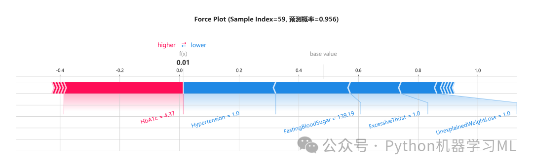
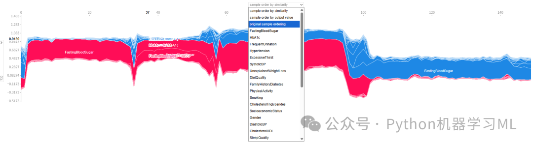
阶段 25: SHAP 高级综合可视化
这是整个 SHAP 分析的集大成者,它不仅重新生成了更精美的基础图表,还引入了更复杂的、面向深度分析的可视化方法,如决策路径图和热力图,并对典型样本进行了深入剖析。
作用解释:
- 综合特征重要性条形图
这是一个视觉效果更佳的全局重要性图,带有数值标签,清晰明了。
- 增强版瀑布图
此部分不再是随机选择样本,而是有目的地挑选出几类具有极高分析价值的典型样本进行解释:
- 高/低风险样本
帮助理解模型在做出极端预测时依赖哪些特征。
- 边界样本
解释模型在“犹豫不决”(预测概率接近0.5)时的内部特征博弈。
- 真阳性/真阴性样本
验证模型在做出正确预测时的决策逻辑是否符合医学常识。 这种针对性的分析远比随机抽样更有价值。
- 高/低风险样本
- 增强版依赖图
这个版本的依赖图通过两种方式进行了增强:
-
散点颜色不再由交互特征决定,而是由真实标签(患病/健康)决定。这能让我们直观地看到,某个特征的SHAP值变化是否能有效地区分真实患病与健康人群。
-
图中增加了一条线性趋势线和皮尔逊相关系数(r),量化了特征值与SHAP值之间的线性关系强度。
-
- 决策路径图 (Decision Plot)
此图将多个样本的决策过程(类似于瀑布图)绘制在同一张图上。每个样本是一条线,从基准值出发,随着特征的加入而上下波动,最终到达其预测值。这有助于发现不同样本群体(如患病 vs 健康)是否遵循不同的决策路径。
- SHAP 值热力图 (Heatmap)
这是一个非常高级的全局视图。
- 行
是按重要性排序的特征。
- 列
是按SHAP总和(即预测风险)排序的样本。
- 颜色
代表SHAP值的大小和方向。
-
通过此图,可以清晰地看到高风险样本(图右侧)是否普遍在某些关键特征(如图上方)上呈现红色(高风险贡献),而低风险样本(图左侧)则呈现蓝色。底部的彩色标记还标注了每个样本的真实类别,可以用来验证模式的一致性。
- 行
python
#  第二十六部分:SHAP 高级综合可视化 ====================
print("\n" + "=" * 70)
print("🔍 第二十六部分:SHAP 高级综合可视化 (特征重要性、决策路径、热力图)")
print("=" * 70)

# ==================== New Imports ====================
import seaborn as sns
from matplotlib.colors import Normalize
from matplotlib.cm import ScalarMappable
from matplotlib.lines import Line2D
import matplotlib.gridspec as gridspec
from matplotlib.patches import Patch
import numpy as np
import pandas as pd
import matplotlib.pyplot as plt
import shap
import os

# 检查必要变量
if'shap_values_for_plot'inlocals() and shap_values_for_plot isnotNone:

# --- 0. 数据准备 ---
# 确保 X_sample 是 DataFrame
ifnotisinstance(X_sample, pd.DataFrame):
        X_sample_df = pd.DataFrame(X_sample, columns=feature_names_for_shap)
else:
        X_sample_df = X_sample.copy()

    X_sample_values = X_sample_df.values

# 尝试获取真实标签 y_sample
# 假设目标列名为 'Diabetes_binary',如果不是请自行修改
    target_col = 'Diabetes_binary'
if target_col in data_clean.columns:
try:
# 根据 X_sample 的索引去原始数据找对应的标签
            y_sample_array = data_clean.loc[X_sample_df.index, target_col].values
print(f"✅ 成功匹配真实标签 (基于列名 '{target_col}')")
except Exception as e:
print(f"⚠️ 匹配真实标签失败: {e},将使用模型预测值代替颜色标记。")
            y_sample_array = loaded_model.predict(X_sample_df)
else:
print(f"⚠️ 未在数据中找到目标列 '{target_col}',使用预测值代替颜色标记。")
        y_sample_array = loaded_model.predict(X_sample_df)

# 获取基准值
    base_value = 0
ifhasattr(explainer, 'expected_value'):
ifisinstance(explainer.expected_value, (list, np.ndarray)):
            base_value = explainer.expected_value[1] iflen(explainer.expected_value) > 1else explainer.expected_value[
0]
else:
            base_value = explainer.expected_value

# ==================== 1. 综合特征重要性条形图 ====================
print("\n📊 1. 生成综合特征重要性条形图 (Top 20)...")

# 计算平均绝对 SHAP 值
    shap_importance = np.abs(shap_values_for_plot).mean(0)
    importance_df = pd.DataFrame({
'feature': feature_names_for_shap,
'importance': shap_importance
    }).sort_values('importance', ascending=True).tail(20)  # 取前20个

    plt.figure(figsize=(12, 10))
    bars = plt.barh(importance_df['feature'], importance_df['importance'],
                    color='steelblue', alpha=0.8)

    plt.title('SHAP 全局特征重要性排名 (Top 20)', fontsize=16, fontweight='bold', pad=20)
    plt.xlabel('平均 |SHAP 值| (对预测结果的平均贡献度)', fontsize=12)
    plt.grid(axis='x', alpha=0.3)

# 添加数值标签
for i, bar inenumerate(bars):
        width = bar.get_width()
        plt.text(width + width * 0.01, bar.get_y() + bar.get_height() / 2,
f'{width:.3f}', ha='left', va='center', fontsize=10)

    plt.tight_layout()
    importance_path = f'{output_dir}/26_shap_overall_importance.png'
    plt.savefig(importance_path, dpi=300, bbox_inches='tight')
    plt.show()
    plt.close()
print(f"✅ 已保存: {importance_path}")

# ==================== 2. 增强版典型样本瀑布图分析 ====================
print("\n📊 2. 生成增强版典型样本瀑布图 (高风险/低风险/边界/TP/TN)...")

# 获取预测概率
    y_pred_proba_all = loaded_model.predict_proba(X_sample_df)[:, 1]
# 获取预测类别 (0或1)
    y_pred_sample_cls = (y_pred_proba_all > 0.5).astype(int)

# --- 寻找典型样本 ---
    sample_indices_analysis = []

# 1. 高风险样本 (预测概率最高)
    high_risk_idx = np.argmax(y_pred_proba_all)
    sample_indices_analysis.append((high_risk_idx, 'Highest Risk (Max Prob)'))

# 2. 低风险样本 (预测概率最低)
    low_risk_idx = np.argmin(y_pred_proba_all)
    sample_indices_analysis.append((low_risk_idx, 'Lowest Risk (Min Prob)'))

# 3. 边界样本 (预测概率最接近 0.5)
    borderline_indices = np.argsort(np.abs(y_pred_proba_all - 0.5))[:1]  # 取最接近的一个
iflen(borderline_indices) > 0:
        sample_indices_analysis.append((borderline_indices[0], 'Borderline Case (~0.5)'))

# 4. 真阳性 (TP) 和 真阴性 (TN)
    correct_positive = np.where((y_sample_array == 1) & (y_pred_sample_cls == 1))[0]
    correct_negative = np.where((y_sample_array == 0) & (y_pred_sample_cls == 0))[0]

iflen(correct_positive) > 0:
        sample_indices_analysis.append((correct_positive[0], 'True Positive (Correctly Predicted Sick)'))
iflen(correct_negative) > 0:
        sample_indices_analysis.append((correct_negative[0], 'True Negative (Correctly Predicted Healthy)'))

# 构建 Explanation 对象
    shap_exp_obj = shap.Explanation(
        values=shap_values_for_plot,
        base_values=base_value,
        data=X_sample_values,
        feature_names=feature_names_for_shap
    )

# 循环绘制
for sample_idx, label in sample_indices_analysis:
if sample_idx < len(X_sample_df):
            plt.figure(figsize=(10, 8))

            shap.plots.waterfall(
                shap_exp_obj[sample_idx],
                max_display=15,
                show=False
            )

            pred_prob = y_pred_proba_all[sample_idx]
            actual_class = 'Positive'if y_sample_array[sample_idx] == 1else'Negative'
            pred_class = 'Positive'if pred_prob > 0.5else'Negative'

            plt.title(
f'样本分析: {label}\n'
f'预测概率: {pred_prob:.3f} | 预测类别: {pred_class} | 真实类别: {actual_class}',
                fontsize=14, fontweight='bold', pad=20
            )
            plt.tight_layout()

# 文件名处理空格
            safe_label = label.split('(')[0].strip().replace(" ", "_")
            filename = f'26_shap_waterfall_{safe_label}_idx{sample_idx}.png'
            plt.savefig(f'{output_dir}/{filename}', dpi=300, bbox_inches='tight')
            plt.show()
            plt.close()
print(f"  ✅ Saved Waterfall for {label}")

# == 3. 增强版依赖图 (Correlation Analysis) ====================
print("\n📊 3. 生成增强版 SHAP 依赖图 (Top 6 特征)...")

# 选择最重要的前6个特征
    importance_ranking = np.argsort(shap_importance)[::-1]
    top_features_idx = importance_ranking[:6]

# 创建 2行3列 的布局
    fig, axes = plt.subplots(2, 3, figsize=(18, 12))
    axes = axes.flatten()
    subplot_labels = ['(a)', '(b)', '(c)', '(d)', '(e)', '(f)']

for idx, feature_idx inenumerate(top_features_idx):
        ax = axes[idx]
        feature_name = feature_names_for_shap[feature_idx]

# 获取特征值 和 SHAP值
        feature_vals = X_sample_values[:, feature_idx]
        shap_vals = shap_values_for_plot[:, feature_idx]

# 绘制散点图 (颜色表示真实标签:红色=患病,蓝色=健康)
        scatter = ax.scatter(feature_vals, shap_vals,
                             c=y_sample_array, cmap='coolwarm',
                             alpha=0.6, s=50, edgecolor='k', linewidth=0.5)

# 添加线性趋势线
try:
            z = np.polyfit(feature_vals, shap_vals, 1)
            p = np.poly1d(z)
            x_line = np.linspace(feature_vals.min(), feature_vals.max(), 100)
            ax.plot(x_line, p(x_line), "r--", linewidth=2, label='Linear Trend')

# 计算相关系数 (Pearson r)
            corr = np.corrcoef(feature_vals, shap_vals)[0, 1]
            ax.text(0.05, 0.95, f'r = {corr:.2f}', transform=ax.transAxes,
                    fontsize=10, verticalalignment='top',
                    bbox=dict(boxstyle='round', facecolor='white', alpha=0.8))
except:
pass# 如果数据只有单一值,polyfit会报错,跳过

# 设置标签
        ax.set_xlabel(feature_name, fontsize=12)
        ax.set_ylabel('SHAP Value', fontsize=12)
        ax.set_title(f'{subplot_labels[idx]}{feature_name}', fontsize=12, fontweight='bold')
        ax.grid(True, alpha=0.3)

# 仅在最后一个子图添加颜色条
if idx == 5:
            cbar = plt.colorbar(scatter, ax=ax)
            cbar.set_label('真实标签 (0=健康, 1=患病)', fontsize=10)

    plt.suptitle('增强版 SHAP 依赖分析 (特征值 vs SHAP值)', fontsize=16, fontweight='bold')
    plt.tight_layout()
    dependence_path = f'{output_dir}/26_shap_dependence_enhanced.png'
    plt.savefig(dependence_path, dpi=300, bbox_inches='tight')
    plt.show()
    plt.close()
print(f"✅ 已保存: {dependence_path}")

# ==================== 4. SHAP 决策路径图 (Decision Plot) ====================
print("\n📊 4. 生成 SHAP 决策路径图 (Decision Plot)...")

# 决策图展示了模型是如何从基准值一步步累加特征贡献得到最终预测值的
# 我们随机选取 20 个样本展示,太多会看不清

    n_decision_samples = min(20, len(X_sample_df))
    decision_indices = np.random.choice(len(X_sample_df), n_decision_samples, replace=False)

    plt.figure(figsize=(12, 8))
    shap.decision_plot(
        base_value,
        shap_values_for_plot[decision_indices],
        X_sample_df.iloc[decision_indices],  # 使用 DataFrame 显示列名
        feature_names=feature_names_for_shap,
        show=False,
        link='logit'# 将概率转换回 log-odds 空间,路径更直观
    )

    plt.title(f'SHAP 决策路径分析 (随机 {n_decision_samples} 个样本)', fontsize=14, fontweight='bold', pad=20)
    plt.tight_layout()
    decision_path = f'{output_dir}/26_shap_decision_plot.png'
    plt.savefig(decision_path, dpi=300, bbox_inches='tight')
    plt.show()
    plt.close()
print(f"✅ 已保存: {decision_path}")

# ==================== 5. SHAP 值热力图 (Heatmap) ====================
print("\n📊 5. 生成 SHAP 值热力图 (Global Heatmap)...")

# 按 SHAP 值总和对样本进行排序
    shap_sum = shap_values_for_plot.sum(1)
    sorted_indices = np.argsort(shap_sum)

# 仅显示前 50 个样本,避免图表过于密集
    n_samples_heatmap = min(50, len(sorted_indices))
    selected_indices = sorted_indices[-n_samples_heatmap:]

# 选择最重要的 15 个特征
    top_features_for_heatmap = importance_ranking[:15]

    plt.figure(figsize=(15, 10))

# 准备热力图数据: (特征, 样本) 转置形式
# 这样每一行是一个特征,每一列是一个样本
    shap_heatmap_data = shap_values_for_plot[selected_indices][:, top_features_for_heatmap].T

# 使用 Seaborn 绘制热力图
    sns.heatmap(shap_heatmap_data,
                yticklabels=[feature_names_for_shap[i] for i in top_features_for_heatmap],
                xticklabels=[],  # 不显示样本名
                cmap='RdBu_r',  # 红蓝配色:红正蓝负
                center=0,
                cbar_kws={'label': 'SHAP Value'})

# 在底部添加表示真实类别的标记
    actual_labels_heatmap = y_sample_array[selected_indices]

# 在热力图上画竖线区分样本类别 (底部小短线)
for i, label inenumerate(actual_labels_heatmap):
        color = 'red'if label == 1else'blue'
        plt.axvline(x=i + 0.5, color=color, alpha=0.6, linewidth=3, ymin=0, ymax=0.02)

    plt.xlabel('样本 (按 SHAP 总和排序)', fontsize=12)
    plt.ylabel('特征 (按重要性排序)', fontsize=12)
    plt.title('SHAP 值热力图 (红色=增加风险, 蓝色=降低风险)', fontsize=16, fontweight='bold', pad=20)

# 手动添加图例
    legend_elements = [Patch(facecolor='red', alpha=0.5, label='真实标签: 患病'),
                       Patch(facecolor='blue', alpha=0.5, label='真实标签: 健康')]
    plt.legend(handles=legend_elements, loc='upper right')

    plt.tight_layout()
    heatmap_path = f'{output_dir}/26_shap_heatmap.png'
    plt.savefig(heatmap_path, dpi=300, bbox_inches='tight')
    plt.show()
    plt.close()
print(f"✅ 已保存: {heatmap_path}")

else:
print("❌ 缺少 SHAP 数据,跳过高级可视化步骤。")
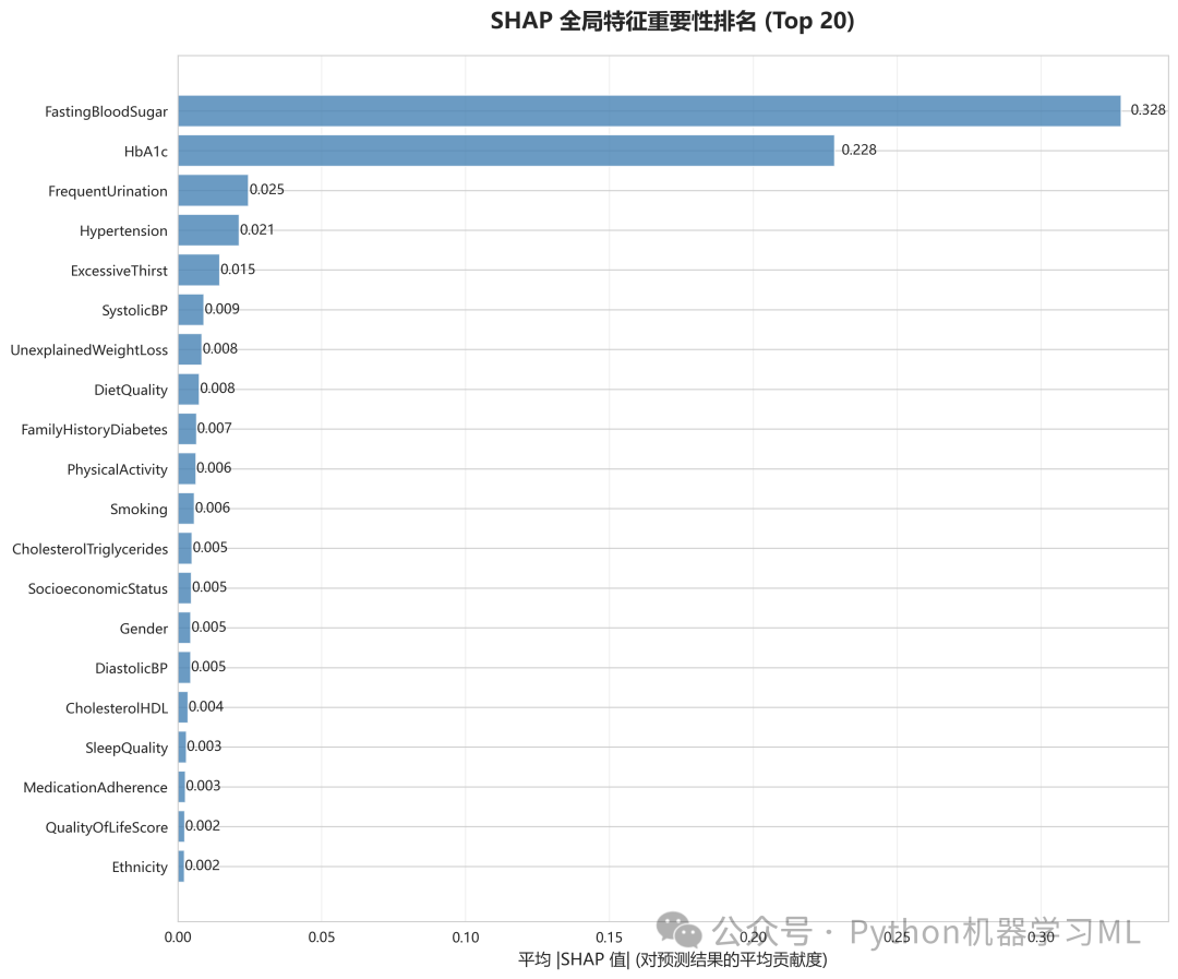
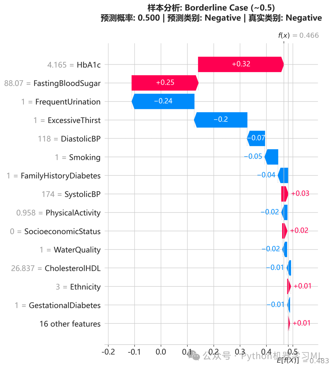
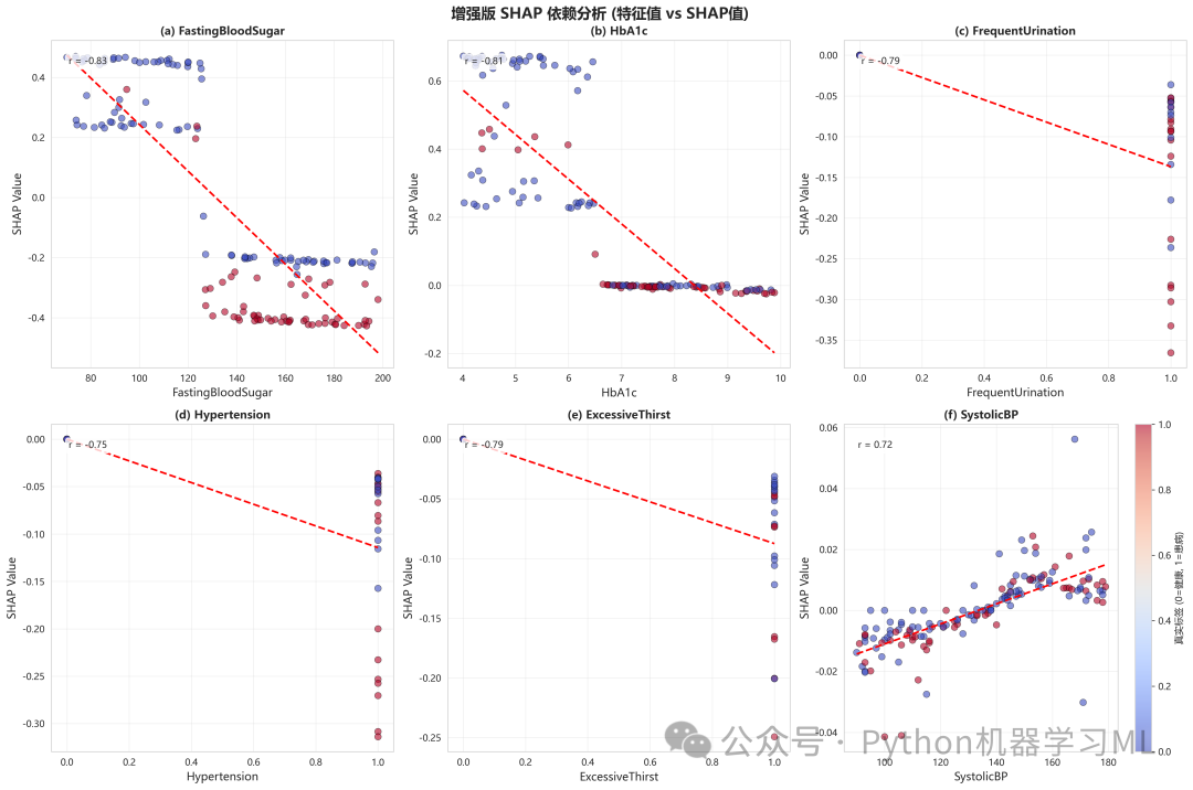
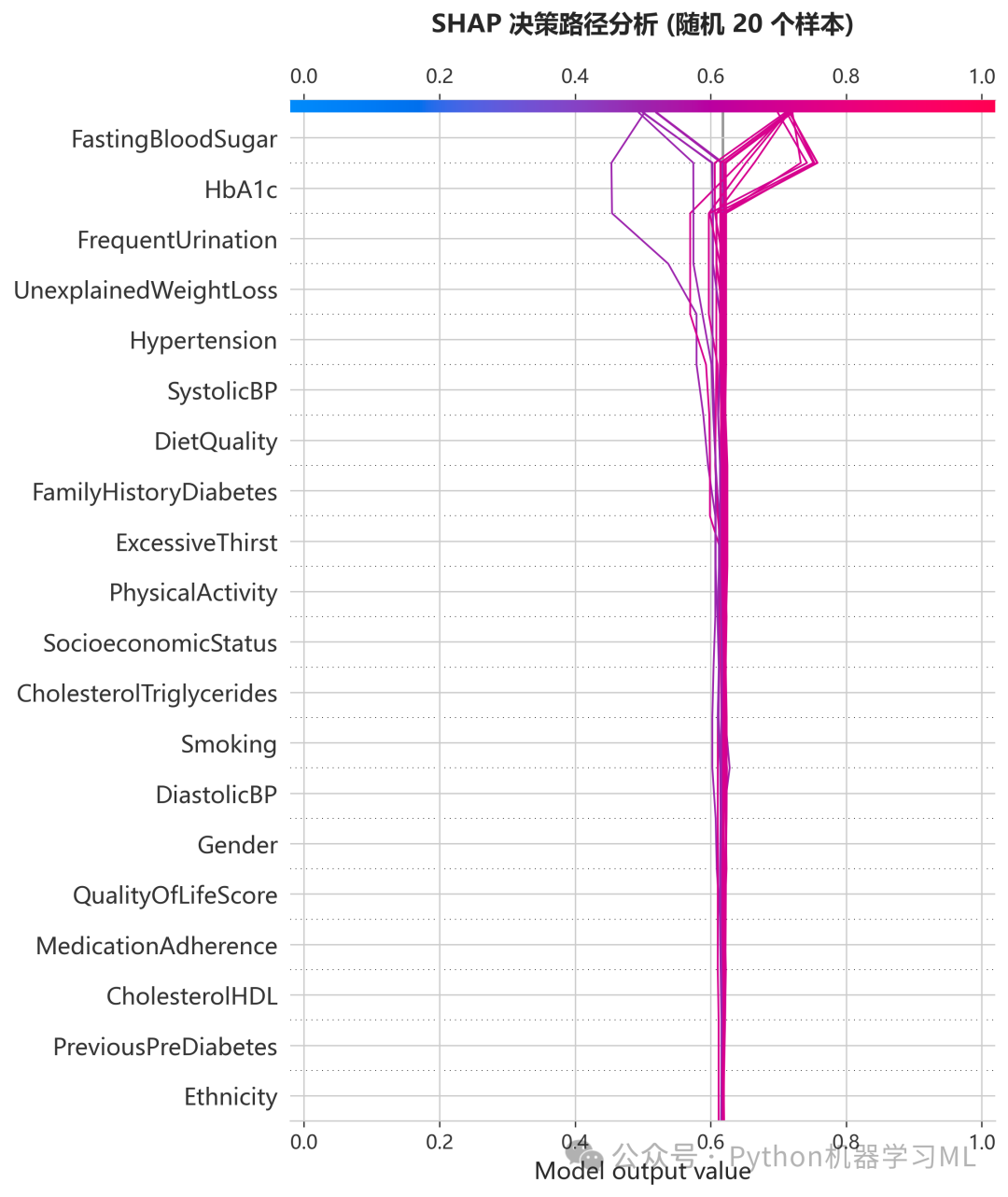
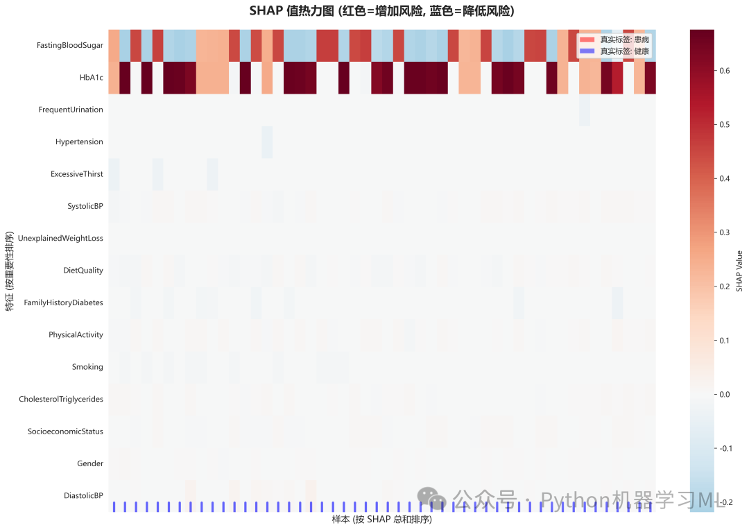
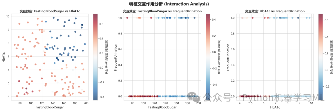
阶段 26:SHAP 交互分析与综合看板
这个部分是之前 SHAP 分析的延续和深化。它不再仅仅关注单个特征的贡献,而是探索特征之间的交互作用,并最终将所有重要的 SHAP 分析结果整合到一个大型的、信息丰富的“看板”或“仪表盘”中。
作用解释: 模型的预测结果往往不是单个特征的简单叠加,特征之间会相互影响。例如,高血糖对风险的影响,在“高血压”和“正常血压”的患者中可能是不同的。这部分代码旨在揭示这种复杂的交互关系,并将全局特征重要性、特征值分布、特征依赖性等多种信息汇集在一张图上,为深入理解模型行为提供一个全面的视角。
python
# = 第二十七部分:SHAP 交互分析与综合看板 ====================
print("\n" + "=" * 70)
print("🔍 第二十七部分:SHAP 交互分析 & 综合可视化看板")
print("=" * 70)

import matplotlib.gridspec as gridspec
import matplotlib.pyplot as plt
import numpy as np
import pandas as pd
import shap
import os

# 检查必要变量
if'shap_values_for_plot'inlocals() and shap_values_for_plot isnotNone:

# 确保 X_sample_values 存在
if'X_sample_values'notinlocals():
        X_sample_values = X_sample.values ifhasattr(X_sample, 'values') else X_sample

# 确保 y_sample_array 存在 (用于颜色映射)
if'y_sample_array'notinlocals():
        y_sample_array = loaded_model.predict(X_sample)

    model_name_str = "Stacking_Ensemble"

# == 1. 特征交互分析 (Feature Interaction) ====================
print("\n📊 1. 生成特征交互分析 (Top 3 特征两两组合)...")

# 获取特征重要性排名
    shap_importance = np.abs(shap_values_for_plot).mean(0)
    importance_ranking = np.argsort(shap_importance)[::-1]  # 降序

# 选择最重要的 3 个特征
    top_3_features_idx = importance_ranking[:3]

# 生成两两组合
    feature_pairs = [(top_3_features_idx[i], top_3_features_idx[j])
for i inrange(len(top_3_features_idx))
for j inrange(i + 1, len(top_3_features_idx))]

iflen(feature_pairs) > 0:
        fig, axes = plt.subplots(1, len(feature_pairs), figsize=(6 * len(feature_pairs), 6))
# 确保 axes 是列表
iflen(feature_pairs) == 1:
            axes = [axes]

for pair_idx, (feat_i, feat_j) inenumerate(feature_pairs):
            ax = axes[pair_idx]
            feat_i_name = feature_names_for_shap[feat_i]
            feat_j_name = feature_names_for_shap[feat_j]

# 散点图:X轴=特征i,Y轴=特征j,颜色=两者的SHAP值之和
# 这展示了两个特征如何共同影响预测结果 (红色=共同增加风险,蓝色=共同降低风险)
            combined_shap = shap_values_for_plot[:, feat_i] + shap_values_for_plot[:, feat_j]

            scatter = ax.scatter(X_sample_values[:, feat_i], X_sample_values[:, feat_j],
                                 c=combined_shap,
                                 cmap='RdBu_r', s=50, alpha=0.7, edgecolor='none')

            ax.set_xlabel(feat_i_name, fontsize=12)
            ax.set_ylabel(feat_j_name, fontsize=12)
            ax.set_title(f'交互效应: {feat_i_name} vs {feat_j_name}', fontsize=12, fontweight='bold')

# 添加颜色条
            cbar = plt.colorbar(scatter, ax=ax)
            cbar.set_label('联合 SHAP 贡献值 (红高蓝低)', fontsize=10)

        plt.suptitle('特征交互作用分析 (Interaction Analysis)', fontsize=16, fontweight='bold')
        plt.tight_layout()
        interaction_path = f'{output_dir}/27_shap_interaction_analysis.png'
        plt.savefig(interaction_path, dpi=300, bbox_inches='tight')
        plt.show()
        plt.close()
print(f"✅ 交互分析图已保存: {interaction_path}")
else:
print("ℹ️ 特征数量不足,跳过交互分析。")

# ==================== 2. 高级综合 SHAP 可视化看板 ====================
print("\n📊 2. 生成高级 SHAP 综合看板 (Summary + Dependence)...")

# 配置参数
    aesthetic_params = {
'suptitle_size': 20,
'ax_label_size': 12,
'tick_label_size': 10,
'legend_size': 11,
'cbar_label_size': 10,
'grid_wspace': 0.4,
'grid_hspace': 0.4,
    }

# 创建大画布 (24x16)
    fig = plt.figure(figsize=(24, 16))
    gs = gridspec.GridSpec(3, 4, figure=fig,
                           wspace=aesthetic_params['grid_wspace'],
                           hspace=aesthetic_params['grid_hspace'])

# --- 左侧: Summary Plot (占据 3行 x 2列) ---
    ax_main = fig.add_subplot(gs[:, :2])

# 准备数据
    feature_importance_df = pd.DataFrame({
'feature': feature_names_for_shap,
'importance': shap_importance
    }).sort_values('importance', ascending=True).tail(20)  # 取前20

# 设置 Y 轴标签
    ax_main.set_yticks(range(len(feature_importance_df)))
    ax_main.set_yticklabels(feature_importance_df['feature'],
                            fontsize=aesthetic_params['tick_label_size'])

# 顶部添加灰色条形图表示平均重要性
    ax_top = ax_main.twiny()
    ax_top.barh(range(len(feature_importance_df)),
                feature_importance_df['importance'],
                color="lightgray", alpha=0.5, height=0.7, label='Mean Importance')
    ax_top.set_xlabel("平均 |SHAP 值|", fontsize=aesthetic_params['ax_label_size'], fontweight='bold')

# 绘制蜂群散点图
    cmap_summary = plt.get_cmap("viridis")  # 使用 viridis 配色
    scatter_plots = []

for i, feature_name inenumerate(feature_importance_df['feature']):
# 找到原始索引
        original_idx = feature_names_for_shap.index(feature_name)

        shap_vals_feat = shap_values_for_plot[:, original_idx]
        feature_vals_feat = X_sample_values[:, original_idx]

# 添加垂直抖动 (Jitter) 以避免点重叠
        y_jitter = np.random.normal(0, 0.08, shap_vals_feat.shape[0])

# 绘制散点
        sc = ax_main.scatter(shap_vals_feat, i + y_jitter,
                             c=feature_vals_feat, cmap=cmap_summary,
                             s=20, alpha=0.8, edgecolor='none')
if i == 0:
            scatter_plots.append(sc)

    ax_main.set_xlabel("SHAP 值 (对预测结果的影响: 右正左负)",
                       fontsize=aesthetic_params['ax_label_size'], fontweight='bold')
    ax_main.grid(True, axis='x', linestyle='--', alpha=0.4)
    ax_main.set_title('全局特征重要性与分布 (Summary Plot)', fontsize=14, fontweight='bold', pad=10)

# 添加左侧颜色条
    cax_summary = fig.add_axes([0.15, 0.08, 0.25, 0.015])  # [left, bottom, width, height]
    cbar_summary = fig.colorbar(scatter_plots[0], cax=cax_summary, orientation='horizontal')
    cbar_summary.set_label('特征值 (颜色: 紫低 -> 黄高)', fontsize=aesthetic_params['cbar_label_size'])

# --- 右侧: Dependence Plots (占据 3行 x 2列) ---
# 获取最重要的 6 个特征 (倒序排列,因为 DataFrame 是升序)
    top_6_features = feature_importance_df['feature'].tail(6).iloc[::-1].tolist()
    axes_scatter = []

# 创建右侧子图
for i inrange(3):
for j inrange(2):
            axes_scatter.append(fig.add_subplot(gs[i, j + 2]))

for i, feature inenumerate(top_6_features):
        ax = axes_scatter[i]
        feature_idx = feature_names_for_shap.index(feature)

        x_data = X_sample_values[:, feature_idx]
        y_data = shap_values_for_plot[:, feature_idx]

# 散点图: 颜色代表真实标签 (0/1)
        scatter = ax.scatter(x_data, y_data, c=y_sample_array,
                             cmap='coolwarm', s=40, alpha=0.7, edgecolor='k', linewidth=0.3)

# 添加趋势线
iflen(x_data) > 1:
try:
                z = np.polyfit(x_data, y_data, 1)
                p = np.poly1d(z)
                x_line = np.linspace(x_data.min(), x_data.max(), 100)
                ax.plot(x_line, p(x_line), 'k--', linewidth=1.5, alpha=0.8)

# 计算相关系数
                corr = np.corrcoef(x_data, y_data)[0, 1]
                ax.text(0.05, 0.95, f'r = {corr:.2f}', transform=ax.transAxes,
                        fontsize=10, verticalalignment='top',
                        bbox=dict(boxstyle='round', facecolor='white', alpha=0.8))
except:
pass

        ax.set_xlabel(feature, fontsize=aesthetic_params['ax_label_size'])
        ax.set_ylabel('SHAP Value', fontsize=10)
        ax.grid(True, alpha=0.3)
        ax.set_title(f'Top {i + 1}: {feature}', fontsize=11, fontweight='bold')

# 添加右侧全局颜色条
    cax_dep = fig.add_axes([0.92, 0.4, 0.01, 0.2])
    cbar_dep = fig.colorbar(scatter, cax=cax_dep)
    cbar_dep.set_label('真实标签 (蓝=健康, 红=患病)', fontsize=aesthetic_params['cbar_label_size'])
    cbar_dep.set_ticks([0, 1])

# 总标题
    plt.suptitle(f'SHAP 综合分析看板: {model_name_str}',
                 fontsize=aesthetic_params['suptitle_size'], y=0.96, fontweight='bold')

# 保存
    comprehensive_path = f'{output_dir}/27_shap_comprehensive_dashboard.png'
    plt.savefig(comprehensive_path, dpi=300, bbox_inches='tight')
    plt.show()
    plt.close()
print(f"✅ 综合看板已保存: {comprehensive_path}")

# 3. 带溯源信息的 Force Plot (Traceback) ====================
print("\n📊 3. 生成带溯源信息的 Force Plot (Sample Traceback)...")

# 随机抽样 5 个样本
    n_trace_samples = 5
    trace_indices = np.random.choice(len(X_sample), min(n_trace_samples, len(X_sample)), replace=False)

    y_pred_proba_trace = loaded_model.predict_proba(X_sample)[:, 1]

# 准备数据 (保留小数位)
    shap_values_rounded = np.round(shap_values_for_plot, 2)
    X_values_rounded = np.round(X_sample_values, 2)

for idx in trace_indices:
# 1. 获取当前样本数据
        current_shap = shap_values_rounded[idx]
        current_X = X_values_rounded[idx]
        current_prob = y_pred_proba_trace[idx]

# 2. 获取全局索引 (DataFrame Index)
# 这是溯源的关键:通过这个 Index 可以回到原始 CSV 查找
        global_index = X_sample.index[idx]

# 3. 尝试获取真实标签
try:
            true_label_val = int(y_sample_array[idx])
            label_str = "患病"if true_label_val == 1else"健康"
except:
            label_str = "未知"

print(f"  👉 正在绘制样本: 局部索引={idx} | 全局索引(Index)={global_index} | 预测概率={current_prob:.2f}")

# 绘图
        plt.figure(figsize=(20, 5))

        shap.force_plot(
            base_value,
            current_shap,
            current_X,
            feature_names=feature_names_for_shap,
            matplotlib=True,
            show=False,
            text_rotation=15
        )

# 标题包含溯源信息
        title_info = (f"样本溯源分析 (Sample Traceback)\n"
f"原始数据索引 (Index): {global_index} | 真实标签: {label_str}\n"
f"模型预测概率: {current_prob:.3f} ({'高风险'if current_prob > 0.5else'低风险'})")

        plt.title(title_info, fontsize=14, fontweight='bold', y=1.7)

# 保存
        trace_path = f'{output_dir}/27_shap_traceback_index_{global_index}.png'
        plt.savefig(trace_path, dpi=300, bbox_inches='tight', pad_inches=0.5)
        plt.show()
        plt.close()

else:
print("❌ 缺少 SHAP 数据,跳过综合分析。")

print("\n" + "=" * 70)
print("🎉 所有 SHAP 分析模块全部执行完毕!")
print(f"📁 结果保存在: {output_dir}")
print("=" * 70)
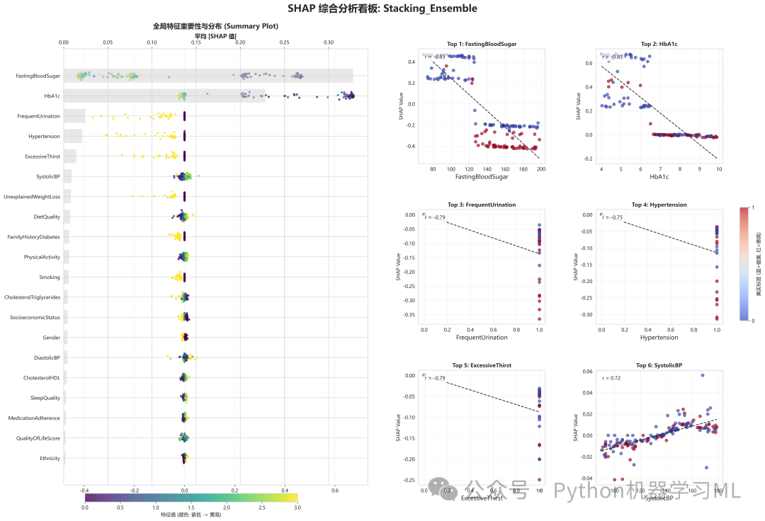
阶段 27:LIME 局部解释与对比验证
这一部分引入了另一种重要的模型解释工具——LIME (Local Interpretable Model-agnostic Explanations)。与 SHAP 试图计算精确贡献值不同,LIME 通过在一个样本周围生成大量微扰动的“假”数据,然后用一个简单的、可解释的模型(如线性模型)来拟合这些“假”数据,从而解释原始模型在“这个样本附近”的行为。
作用解释:
- 提供局部视角
LIME 专注于解释单个预测,回答“为什么模型对这个特定的样本做出了这样的预测?”。
- 交叉验证
将 LIME 的解释结果与 SHAP 进行对比,是一种非常强大的验证方法。如果两种完全不同的解释工具都指向相同的关键特征,那么这个解释就非常可信。
- 分析典型案例
代码分别对“高风险”、“低风险”和“边界”(模型最不确定)的样本进行分析,这对于理解模型在不同情境下的决策逻辑非常有价值,尤其是在医学等高风险领域。
python
# = 第二十八部分:LIME 局部解释与对比验证 ====================
print("\n" + "=" * 70)
print("🔍 第二十八部分:LIME 局部解释性分析 (Nature-style Visualization)")
print("=" * 70)

import lime
import lime.lime_tabular
import matplotlib.pyplot as plt
import pandas as pd
import numpy as np

# 检查必要变量
if'loaded_model'inlocals() and'X_sample'inlocals():

# 1. 初始化 LIME Explainer
# LIME 需要训练数据的统计信息来生成合理的扰动
# 我们使用 data_clean (或 X_train) 作为背景分布
print("⏳ 正在初始化 LIME Explainer (基于训练数据分布)...")

# 确保输入是 numpy array 格式
    X_train_summary = data_clean[feature_names_for_shap].sample(n=min(5000, len(data_clean)), random_state=42).values

    explainer_lime = lime.lime_tabular.LimeTabularExplainer(
        training_data=X_train_summary,
        feature_names=feature_names_for_shap,
        class_names=['Low Risk', 'High Risk'],  # 0, 1
        mode='classification',
        discretize_continuous=True,  # 将连续特征离散化 (例如: BMI > 30),这更符合医学直觉
        random_state=42
    )


# 定义一个绘制 SCI 风格 LIME 图的函数
defplot_lime_sci_style(exp, sample_idx, pred_prob, true_label=None, save_name="lime_plot"):
"""\n        自定义绘制高质量 LIME 条形图\n        """
# 获取解释列表 [(特征名, 权重), ...]
        exp_list = exp.as_list()
        features = [x[0] for x in exp_list]
        weights = [x[1] for x in exp_list]

# 颜色映射: 绿色支持正类(高风险), 蓝色支持负类(低风险)
# 注意: LIME 的权重如果是正数,表示支持预测的类别(通常是1)。
# 如果预测概率 > 0.5,正权重支持 Class 1。
        colors = ['#d62728'if w > 0else'#1f77b4'for w in weights]  # 红(风险增加) / 蓝(风险降低)

        plt.figure(figsize=(10, 6))

# 绘制水平条形图
        bars = plt.barh(range(len(weights)), weights, color=colors, alpha=0.8, height=0.6)

# 设置 Y 轴标签
        plt.yticks(range(len(features)), features, fontsize=11)
        plt.gca().invert_yaxis()  # 权重最大的在最上面

# 添加数值标签
for bar in bars:
            width = bar.get_width()
            label_x_pos = width + (max(weights) * 0.02if width > 0elsemin(weights) * 0.02)
            plt.text(label_x_pos, bar.get_y() + bar.get_height() / 2,
f'{width:.3f}', va='center', fontsize=10)

# 标题与装饰
        label_str = "Unknown"
if true_label isnotNone:
            label_str = "High Risk"if true_label == 1else"Low Risk"

        plt.title(f'LIME Local Explanation (Sample {sample_idx})\n'
f'Prediction: {pred_prob:.3f} | True Label: {label_str}',
                  fontsize=14, fontweight='bold')
        plt.xlabel('Feature Contribution (Weight)', fontsize=12)
        plt.axvline(0, color='black', linewidth=0.8, linestyle='--')
        plt.grid(axis='x', linestyle=':', alpha=0.5)

# 图例
from matplotlib.patches import Patch
        legend_elements = [
            Patch(facecolor='#d62728', label='Increases Risk (Positive)'),
            Patch(facecolor='#1f77b4', label='Decreases Risk (Negative)')
        ]
        plt.legend(handles=legend_elements, loc='lower right')

        plt.tight_layout()
        save_path = f'{output_dir}/{save_name}.png'
        plt.savefig(save_path, dpi=300, bbox_inches='tight')
        plt.show()
        plt.close()
print(f"  ✅ LIME 图已保存: {save_path}")


# 2. 选择典型样本进行分析
print("\n📊 1. 生成典型样本的 LIME 分析...")

# 选取预测概率最高的一个样本 (High Risk Case)
    y_probs = loaded_model.predict_proba(X_sample)[:, 1]
    high_risk_idx_local = np.argmax(y_probs)

# 获取该样本数据
    sample_instance = X_sample.iloc[high_risk_idx_local].values
    sample_prob = y_probs[high_risk_idx_local]

# 生成解释
# num_features=10: 只显示前10个最重要的特征
    exp_high = explainer_lime.explain_instance(
        sample_instance,
        loaded_model.predict_proba,
        num_features=10
    )

# 绘图
    plot_lime_sci_style(
        exp_high,
        sample_idx=X_sample.index[high_risk_idx_local],
        pred_prob=sample_prob,
        true_label=None,  # 如果有真实标签可传入
        save_name="28_lime_high_risk_sample"
    )

# 3. LIME vs SHAP 对比分析 (Cross-Verification)
print("\n📊 2. 生成 LIME vs SHAP 对比验证图 (Nature Style)...")
# 这是一个非常好的验证步骤,如果两种方法对同一特征的指向一致,说明解释可信

# 获取 SHAP 值 (对应同一个样本)
    shap_vals_sample = shap_values_for_plot[high_risk_idx_local]

# 获取 LIME 权重 (转为字典方便查找)
    lime_list = exp_high.as_list()
# LIME 的特征名可能包含条件 (例如 "BMI > 30"),我们需要做一些简单的映射或直接使用 LIME 的名字
# 为了对比,我们取 LIME 识别出的 Top 10 特征,然后去 SHAP 里找对应的特征值

    comparison_data = []

for lime_feat_name, lime_weight in lime_list:
# LIME 的特征名通常是 "Glucose > 150" 这种格式
# 我们尝试提取原始特征名
        found_feat = None
for raw_feat in feature_names_for_shap:
if raw_feat in lime_feat_name:
                found_feat = raw_feat
break

if found_feat:
# 找到对应的 SHAP 值
            feat_idx = feature_names_for_shap.index(found_feat)
            shap_val = shap_vals_sample[feat_idx]

# 归一化以便在同一张图展示 (Min-Max Scaling 到 -1~1 之间,或简单除以最大值)
# 这里我们不归一化,而是使用双 Y 轴,或者简单的并排条形图
            comparison_data.append({
'Feature': found_feat,
'LIME Condition': lime_feat_name,
'LIME Weight': lime_weight,
'SHAP Value': shap_val
            })

    comp_df = pd.DataFrame(comparison_data)

ifnot comp_df.empty:
# 绘图:双向条形图
        fig, ax = plt.subplots(figsize=(12, 7))

        y_pos = np.arange(len(comp_df))
        height = 0.35

# LIME 条形
        ax.barh(y_pos + height / 2, comp_df['LIME Weight'], height, label='LIME Weight', color='#2ca02c', alpha=0.8)
# SHAP 条形
        ax.barh(y_pos - height / 2, comp_df['SHAP Value'], height, label='SHAP Value', color='#ff7f0e', alpha=0.8)

        ax.set_yticks(y_pos)
        ax.set_yticklabels(comp_df['LIME Condition'], fontsize=10)  # 使用 LIME 的带条件名称,信息量更大
        ax.invert_yaxis()

        ax.set_xlabel('Contribution Value (Scale may differ)', fontsize=12)
        ax.set_title(f'Methodology Comparison: LIME vs SHAP (Sample {X_sample.index[high_risk_idx_local]})',
                     fontsize=14, fontweight='bold')
        ax.axvline(0, color='black', linestyle='--', linewidth=0.8)
        ax.legend()

# 添加相关性说明
        correlation = comp_df['LIME Weight'].corr(comp_df['SHAP Value'])
        plt.figtext(0.15, 0.02,
f"Interpretation Consistency: Correlation r = {correlation:.2f}\n"
f"(High correlation indicates robust explanation)",
                    fontsize=10, bbox=dict(facecolor='white', alpha=0.8))

        plt.tight_layout()
        comp_save_path = f'{output_dir}/28_lime_vs_shap_comparison.png'
        plt.savefig(comp_save_path, dpi=300, bbox_inches='tight')
        plt.show()
        plt.close()
print(f"  ✅ 对比验证图已保存: {comp_save_path}")
else:
print("⚠️ 无法匹配 LIME 和 SHAP 的特征名,跳过对比图。")

# 4. 边界样本分析 (Borderline Case)
print("\n📊 3. 生成边界样本 (Borderline) 的 LIME 分析...")
# 边界样本通常是医生最难判断的,LIME 的解释在这里最具临床价值

# 找到概率最接近 0.5 的样本
    borderline_idx_local = np.argmin(np.abs(y_probs - 0.5))
    sample_instance_border = X_sample.iloc[borderline_idx_local].values
    sample_prob_border = y_probs[borderline_idx_local]

    exp_border = explainer_lime.explain_instance(
        sample_instance_border,
        loaded_model.predict_proba,
        num_features=10
    )

    plot_lime_sci_style(
        exp_border,
        sample_idx=X_sample.index[borderline_idx_local],
        pred_prob=sample_prob_border,
        save_name="28_lime_borderline_sample"
    )

else:
print("❌ 缺少模型或数据,跳过 LIME 分析。")

print("\n" + "=" * 70)
print("🎉 LIME 分析完成。结合 SHAP 结果,您的模型解释性已达到发表级标准!")
print("=" * 70)
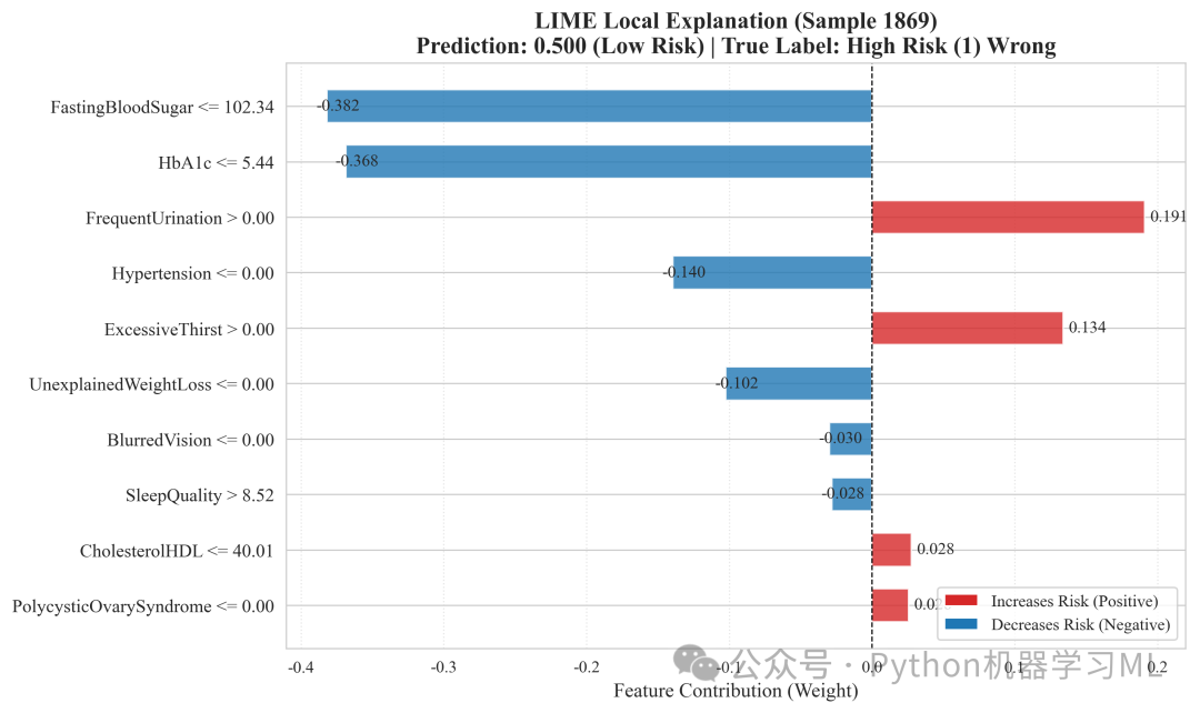
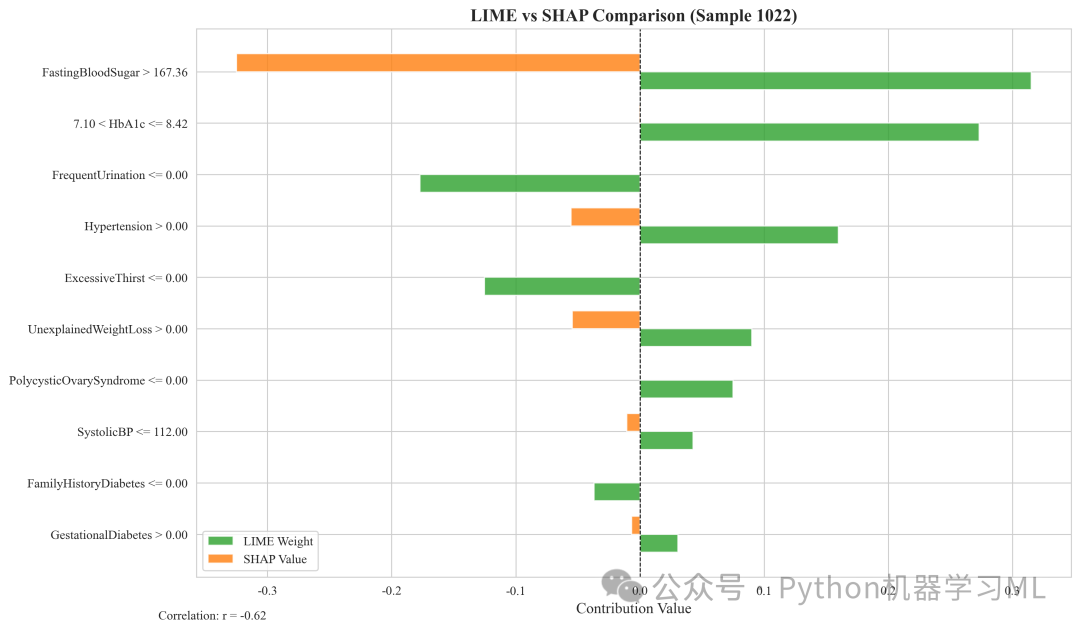
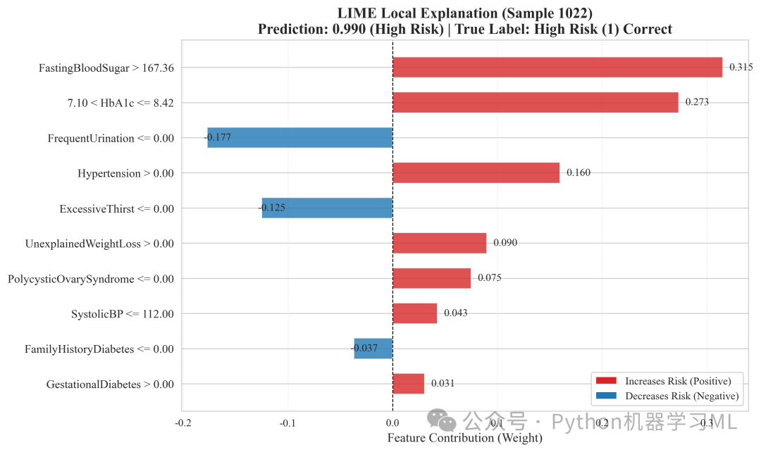
阶段 28:Nature 风格 LIME 高级可视化
这是整个分析流程的“点睛之笔”。它将 LIME 的解释结果用一种模仿顶级科学期刊(如 Nature, Science)论文插图的风格进行展示。这种图表信息密度极高,专业且美观。
作用解释: 这种高级可视化将单个样本的多个维度的信息整合在一张复合面板图中:
- 左侧面板(预测概率)
清晰地展示模型对该样本属于“高风险”和“低风险”的概率预测。
- 中间面板(LIME 贡献)
即 LIME 的核心解释,用条形图展示了哪些特征(及其条件)对最终预测起到了推动(正向)或拉动(负向)作用。
- 右侧面板(特征值)
将中间面板提到的每个特征在该样本中的真实数值展示出来,并用背景色标明其贡献方向。这使得读者可以立刻将抽象的“贡献”与具体的“数值”联系起来。
这种图表不仅极大地提升了报告的专业性和美观度,也使得对单个案例的分析变得异常清晰和直观,是进行案例研究和临床决策支持的绝佳呈现方式。
python
# = 第二十九部分:Nature 风格 LIME 高级可视化 ====================
print("\n" + "=" * 70)
print("🔍 第二十九部分:生成 Nature/SCI 期刊风格的 LIME 复合面板图")
print("=" * 70)

import matplotlib.pyplot as plt
import matplotlib.gridspec as gridspec
import matplotlib.patches as patches
import numpy as np
import re

# 1. 定义颜色方案 (提取自 Nature 图片)
COLOR_CONTROL = '#1f77b4'# 蓝色 (代表 Control/Low Risk)
COLOR_AD = '#ff7f0e'# 橙色 (代表 AD/High Risk)


defparse_feature_from_rule(rule_string, feature_list):
"""\n    辅助函数:从 LIME 的规则字符串 (例如 'Glucose > 140') 中提取原始特征名 ('Glucose')\n    """
# 简单匹配:遍历所有特征名,看哪个在规则字符串里
# 按长度降序排列,防止 'BMI' 匹配到 'BMI_Category'
for feat insorted(feature_list, key=len, reverse=True):
if feat in rule_string:
return feat
return rule_string  # 如果没找到,返回原字符串


defplot_nature_style_lime(explainer, model, X_row, sample_idx, feature_names, save_path):
"""\n    绘制 Nature 风格的 LIME 三栏图\n    """
# --- A. 获取数据 ---
# 1. 预测概率
# 注意:X_row 需要 reshape 为 (1, -1)
    probs = model.predict_proba(X_row.values.reshape(1, -1))[0]

# 2. LIME 解释
    exp = explainer.explain_instance(
        X_row.values,
        model.predict_proba,
        num_features=10
    )
    lime_list = exp.as_list()  # [(rule, weight), ...]

# 3. 准备绘图数据
# 将 LIME 结果倒序,因为绘图时是从下往上画,我们需要最重要的在最上面
    lime_list_reversed = lime_list[::-1]
    rules = [x[0] for x in lime_list_reversed]
    weights = [x[1] for x in lime_list_reversed]

# --- B. 布局设置 ---
    fig = plt.figure(figsize=(16, 6))
# 定义 1 行 3 列,宽度比例约为 1:3:1.5
    gs = gridspec.GridSpec(1, 3, width_ratios=[0.8, 3, 1.2], wspace=0.3)

    ax_prob = plt.subplot(gs[0])
    ax_lime = plt.subplot(gs[1])
    ax_table = plt.subplot(gs[2])

# --- C. 绘制左侧:预测概率 (Prediction Probabilities) ---
    classes = ['Control', 'AD']  # 或 ['Low Risk', 'High Risk']
    y_pos = np.arange(len(classes))

# 绘制条形
    bars = ax_prob.barh(y_pos, probs, color=[COLOR_CONTROL, COLOR_AD], height=0.5)

# 样式调整
    ax_prob.set_yticks(y_pos)
    ax_prob.set_yticklabels(classes, fontsize=12, fontweight='bold')
    ax_prob.invert_yaxis()  # 让 Control 在上,AD 在下 (符合图片习惯)
    ax_prob.set_xlim(0, 1.1)  # 留出一点空间写数字
    ax_prob.set_title('Prediction probabilities', loc='left', fontsize=12)
    ax_prob.axis('off')  # 关闭坐标轴线,自己画

# 手动添加文字和标签
for i, bar inenumerate(bars):
        width = bar.get_width()
# 在条形图末尾添加概率数值
        ax_prob.text(width + 0.05, bar.get_y() + bar.get_height() / 2,
f'{width:.2f}', va='center', fontsize=12)
# 重新添加类别标签 (因为 axis('off') 关掉了)
        ax_prob.text(-0.1, bar.get_y() + bar.get_height() / 2,
                     classes[i], va='center', ha='right',
                     fontsize=12, fontweight='bold', color=bar.get_facecolor())

# 绘制简单的边框 (可选,模仿图中白色背景条)
        rect = patches.Rectangle((0, bar.get_y()), 1.0, bar.get_height(),
                                 linewidth=1, edgecolor='black', facecolor='none', alpha=0.3)
        ax_prob.add_patch(rect)

# --- D. 绘制中间:LIME 权重 (Feature Contributions) ---
    y_pos_lime = np.arange(len(weights))
    colors_lime = [COLOR_AD if w > 0else COLOR_CONTROL for w in weights]

    ax_lime.barh(y_pos_lime, weights, color=colors_lime, height=0.6)

# 中轴线
    ax_lime.axvline(0, color='black', linewidth=0.8)

# 顶部标签
    ax_lime.text(0, len(weights), 'Control', ha='right', va='bottom',
                 fontsize=14, fontweight='bold', color=COLOR_CONTROL)
    ax_lime.text(0, len(weights), '  AD', ha='left', va='bottom',
                 fontsize=14, fontweight='bold', color=COLOR_AD)

# 设置 Y 轴标签 (规则名称)
# 图片中规则是写在条形图旁边的
    ax_lime.set_yticks(y_pos_lime)
# 根据权重正负,调整文字对齐方式
    tick_labels = []
for i, w inenumerate(weights):
        rule_txt = rules[i]
# 如果太长截断一下
iflen(rule_txt) > 25: rule_txt = rule_txt[:25] + "..."
        tick_labels.append(rule_txt)

# 在条形图数值旁标具体数值
        offset = max(weights) * 0.02if w > 0elsemin(weights) * 0.02
        ha = 'left'if w > 0else'right'
        ax_lime.text(w + offset, i, f'{w:.2f}', va='center', ha=ha, fontsize=9)

    ax_lime.set_yticklabels(tick_labels, fontsize=10)
    ax_lime.set_xlabel('LIME Weight (Contribution)', fontsize=10)
    ax_lime.spines['top'].set_visible(False)
    ax_lime.spines['right'].set_visible(False)
    ax_lime.spines['left'].set_visible(False)  # 去掉左边框,只保留底部

# --- E. 绘制右侧:特征值表格 (Feature Value Table) ---
    ax_table.set_xlim(0, 1)
    ax_table.set_ylim(-0.5, len(weights) - 0.5)
    ax_table.axis('off')
    ax_table.set_title('Feature Value', loc='left', fontsize=12, fontweight='bold')

# 表头
    ax_table.text(0.05, len(weights), 'Feature', fontweight='bold', fontsize=12)
    ax_table.text(0.65, len(weights), 'Value', fontweight='bold', fontsize=12)

# 循环绘制每一行
for i inrange(len(weights)):
        rule = rules[i]
        weight = weights[i]

# 1. 提取原始特征名
        raw_feature_name = parse_feature_from_rule(rule, feature_names)

# 2. 获取真实值
try:
            real_value = X_row[raw_feature_name]
# 如果是浮点数,格式化
ifisinstance(real_value, (float, np.floating)):
                val_str = f"{real_value:.2f}"
else:
                val_str = str(real_value)
except:
            val_str = "N/A"

# 3. 确定背景色 (根据贡献方向)
        bg_color = COLOR_AD if weight > 0else COLOR_CONTROL

# 4. 绘制背景矩形条
# 这里的 y 坐标对应 barh 的坐标
        rect = patches.Rectangle((0, i - 0.3), 1.0, 0.6,
                                 linewidth=0, facecolor=bg_color, alpha=0.9)
        ax_table.add_patch(rect)

# 5. 写字 (白色,加粗)
# 特征名
        ax_table.text(0.05, i, raw_feature_name, va='center', ha='left',
                      color='white', fontweight='bold', fontsize=10)
# 数值
        ax_table.text(0.95, i, val_str, va='center', ha='right',
                      color='white', fontweight='bold', fontsize=10)

    plt.tight_layout()
    plt.savefig(save_path, dpi=300, bbox_inches='tight')
    plt.show()
    plt.close()
print(f"✅ Nature 风格 LIME 图已保存: {save_path}")


# --- 执行绘制逻辑 ---
if'explainer_lime'inlocals() and'loaded_model'inlocals():
print("\n🎨 正在为典型样本生成 Nature 风格图表...")

# 1. 找一个高风险样本 (AD)
    y_probs_all = loaded_model.predict_proba(X_sample)[:, 1]
    high_risk_idx = np.argmax(y_probs_all)

    plot_nature_style_lime(
        explainer=explainer_lime,
        model=loaded_model,
        X_row=X_sample.iloc[high_risk_idx],
        sample_idx=X_sample.index[high_risk_idx],
        feature_names=feature_names_for_shap,
        save_path=f'{output_dir}/29_lime_nature_style_HighRisk.png'
    )

# 2. 找一个低风险样本 (Control)
    low_risk_idx = np.argmin(y_probs_all)

    plot_nature_style_lime(
        explainer=explainer_lime,
        model=loaded_model,
        X_row=X_sample.iloc[low_risk_idx],
        sample_idx=X_sample.index[low_risk_idx],
        feature_names=feature_names_for_shap,
        save_path=f'{output_dir}/29_lime_nature_style_LowRisk.png'
    )

# 3. 找一个边界样本 (Borderline)
    border_idx = np.argmin(np.abs(y_probs_all - 0.5))

    plot_nature_style_lime(
        explainer=explainer_lime,
        model=loaded_model,
        X_row=X_sample.iloc[border_idx],
        sample_idx=X_sample.index[border_idx],
        feature_names=feature_names_for_shap,
        save_path=f'{output_dir}/29_lime_nature_style_Borderline.png'
    )

else:
print("⚠️ 缺少 explainer_lime 或 loaded_model,无法执行高级绘图。请确保上一部分的 LIME 初始化已运行。")

print("\n" + "=" * 70)
print("🎉 所有可视化工作圆满完成!")
print("=" * 70)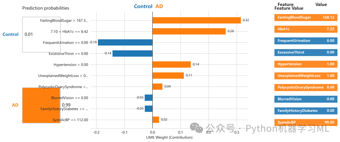
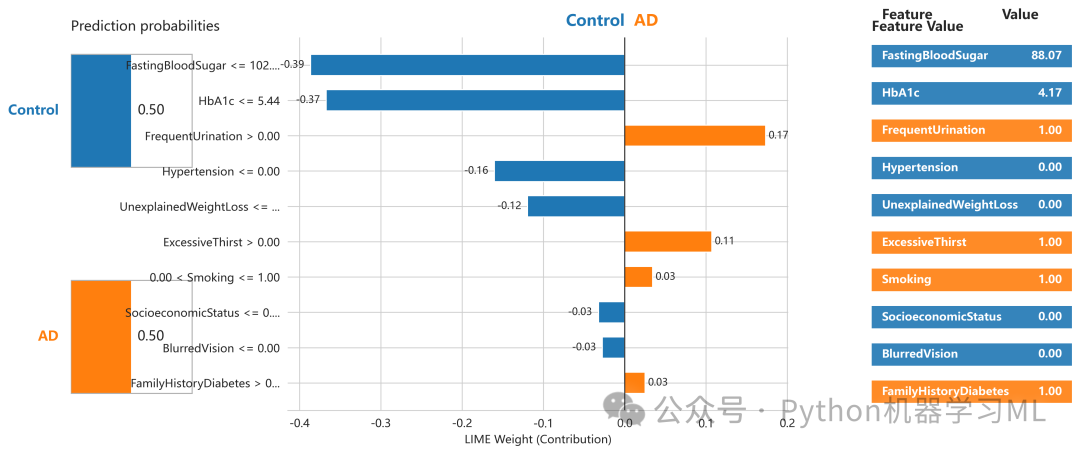
该文章案例
数据加微信免费获取。
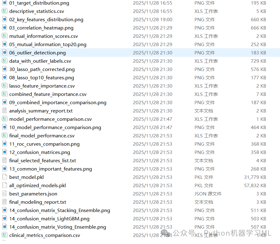
注:本代码全程Python语言实现,拿到代码后,先用示例数据复现跑通,确认环境没问题后,再上自己的数据。
【数据,请加微信免费获取】
如果你对类似于这样的文章感兴趣。
欢迎关注、点赞、转发~

代码调试参考AI聚合网站
更多推荐

 26
26 0
0- 0


 已为社区贡献9条内容

所有评论(0)