概述

在本教程中，我们将学习如何根据一组类别对图像进行分割。分割是指将图像划分为像素组的过程，这些像素组与前景或背景类别（一个包含非目标特征的通用类别）中的目标类别相对应。

具体来说，在这个教程中我们将使用德国作物类型分类的融合数据集。该数据集利用了 Planet 五天合成影像和多边形标签。

我们的任务将是在像素级别预测图像中的作物类型（一种土地利用/土地覆盖形式）。

具体概念

Functional API - 我们将使用 Functional API 实现 UNet，这是一种经典的卷积网络模型，通常用于生物医学图像分割。

该模型包含需要多个输入/输出的层。这需要使用 Functional API。

查看原始论文，Olaf Ronneberger 的《U-Net：用于生物医学图像分割的卷积网络》！

损失函数和指标 - 我们将实现稀疏分类焦点损失函数和准确率。我们还将评估期间生成混淆矩阵，以判断模型的性能。

保存和加载 Keras 模型 - 我们将最佳模型保存到文件中。当未来我们需要进行推理/评估模型时，可以加载模型文件。

通用工作流程

从 Google Drive 加载图像和标签数据集（在上一课中获取和处理）

可视化数据/执行一些探索性数据分析

设置数据管道和预处理

构建模型

训练模型

测试模型

目标

使用 Keras 函数式 API 作为运行 TensorFlow 模型的手段进行实践

体验训练分割模型并监控进度

学习如何使用训练好的分割模型生成预测

设置笔记本

除了我们之前使用的地理空间 Python 依赖项外，我们还将安装并导入一些其他库：tensorflow/examples - 我们仅安装这个库以访问我们用于构建 U-Net 解码器部分的 pix2pix 上采样块

focal-loss - 一个在 Keras 中实现焦点损失函数的 Python 包。焦点损失特别适用于卫星图像以及标记数据集中目标类之间或背景类与目标类之间的类别不平衡。

tf-explain - 一个用于检查网络激活层的 tensorboard 扩展，以便我们可以可视化模型学习的内容。

segmentation-models - 一个实现许多标准、流行的深度学习模型和分割指标的 Keras 库。该库有些过时，但它仍然有用，因为它将 Keras 模型架构和指标专门为分割组织在一个包中。

# install required libraries
!pip install -q git+https://github.com/tensorflow/examples.git
!pip install -q -U tfds-nightly==4.9.2
!pip install -q geopandas==0.13.2
!pip install -q focal-loss==0.0.7
#!pip install -q matplotlib==3.5 # UNCOMMENT if running on LOCAL
!pip install -q scikit-learn==1.2.2
!pip install -q scikit-image==0.19.3
!pip install -q tf-explain==0.3.1
!pip install -q segmentation_models==1.0.1 # we'll use this for pretraining later and for the IOU segmentation performance metric
!pip install -q tensorflow==2.2.1
!pip install -q keras==2.5

# import required libraries
import os, glob, functools, shutil
os.environ["SM_FRAMEWORK"] = "tf.keras"

import numpy as np
import matplotlib.pyplot as plt
import matplotlib as mpl
mpl.rcParams['axes.grid'] = False
mpl.rcParams['figure.figsize'] = (12,12)

from sklearn.model_selection import train_test_split
import matplotlib.image as mpimg
import pandas as pd
from PIL import Image
import geopandas as gpd
from focal_loss import SparseCategoricalFocalLoss
from segmentation_models.metrics import iou_score

import skimage.io as skio
import tensorflow as tf
from tensorflow_examples.models.pix2pix import pix2pix
from tf_explain.callbacks.activations_visualization import ActivationsVisualizationCallback
import tensorflow_datasets as tfds
tfds.disable_progress_bar()

from IPython.display import clear_output
from tqdm.notebook import tqdm
import datetime
from google.colab import drive

准备数据

我们将使用 tf-eo-devseed-processed-outputs 文件夹中的以下文件夹和文件：

tf-eo-devseed-processed-outputs/
├── stacks/
├── stacks_brightened/
├── indices/
├── labels/
├── background_list_train.txt
├── train_list_clean.txt
└── lulc_classes.csv

# set your folders
if 'google.colab' in str(get_ipython()):
    # mount google drive
    drive.mount('/content/gdrive')
    processed_outputs_dir = '/content/gdrive/My Drive/tf-eo-devseed-processed-outputs/'
    user_outputs_dir = '/content/gdrive/My Drive/tf-eo-devseed-user_outputs_dir'
    if not os.path.exists(user_outputs_dir):
        os.makedirs(user_outputs_dir)
    print('Running on Colab')
else:
    processed_outputs_dir = os.path.abspath("./data/tf-eo-devseed-processed-outputs")
    user_outputs_dir = os.path.abspath('./tf-eo-devseed-user_outputs_dir')
    if not os.path.exists(user_outputs_dir):
        os.makedirs(user_outputs_dir)
        os.makedirs(processed_outputs_dir)
    print(f'Not running on Colab, data needs to be downloaded locally at {os.path.abspath(processed_outputs_dir)}')
    
img_dir = os.path.join(processed_outputs_dir,'rasters/tiled/stacks_brightened/') # or os.path.join(processed_outputs_dir,'rasters/tiled/indices/') if using the indices
label_dir = os.path.join(processed_outputs_dir,'rasters/tiled/labels/')

# Move to your user directory in order to write data
%cd $processed_outputs_dir

启用 GPU

本笔记本可以利用 GPU，并且使用 GPU 时效果更好。希望本笔记本正在使用 GPU，我们可以通过以下代码进行检查。

device_name = tf.test.gpu_device_name()
if device_name != '/device:GPU:0':
  raise SystemError('GPU device not found')
print('Found GPU at: {}'.format(device_name))

查看标签

从提供的文档中提取的类名和标识符：https://radiantearth.blob.core.windows.net/mlhub/esa-food-security-challenge/Crops_GT_Brandenburg_Doc.pdf

# Read the classes

data = {'class_names':  ['Background', 'Wheat', 'Rye', 'Barley', 'Oats', 'Corn', 'Oil Seeds', 'Root Crops', 'Meadows', 'Forage Crops'],
        'class_ids': [0, 1, 2, 3, 4, 5, 6, 7, 8, 9]
        }

classes = pd.DataFrame(data)
print(classes)

读取 tensorflow 数据集

现在我们将频谱指数图像和标签瓦片编译成用于 TensorFlow 的训练、验证和测试数据集。

获取用于训练和测试的图像和标签瓦片对列表。

def get_train_test_lists(imdir, lbldir):
  imgs = glob.glob(os.path.join(imdir,"*.png"))
  #print(imgs[0:1])
  dset_list = []
  for img in imgs:
    filename_split = os.path.splitext(img)
    filename_zero, fileext = filename_split
    basename = os.path.basename(filename_zero)
    dset_list.append(basename)

  x_filenames = []
  y_filenames = []
  for img_id in dset_list:
    x_filenames.append(os.path.join(imdir, "{}.png".format(img_id)))
    y_filenames.append(os.path.join(lbldir, "{}.png".format(img_id)))

  print("number of images: ", len(dset_list))
  return dset_list, x_filenames, y_filenames

train_list, x_train_filenames, y_train_filenames = get_train_test_lists(img_dir, label_dir)

检查背景瓦片的比例。这需要一些时间。所以，运行一次后，你可以通过加载保存的结果来跳过这一步。

skip = True

if not skip:
  background_list_train = []
  for i in train_list:
      # read in each labeled images
      # print(os.path.join(label_dir,"{}.png".format(i)))
      img = np.array(Image.open(os.path.join(label_dir,"{}.png".format(i))))
      # check if no values in image are greater than zero (background value)
      if img.max()==0:
          background_list_train.append(i)

  print("Number of background images: ", len(background_list_train))

  with open(os.path.join(processed_outputs_dir,'background_list_train.txt'), 'w') as f:
    for item in background_list_train:
        f.write("%s\n" % item)

else:
  background_list_train = [line.strip() for line in open("background_list_train.txt", 'r')]
  print("Number of background images: ", len(background_list_train))

我们将只保留总量的 10%。过多的背景瓦片会导致一种形式的类别不平衡。

background_removal = len(background_list_train) * 0.9
train_list_clean = [y for y in train_list if y not in background_list_train[0:int(background_removal)]]

x_train_filenames = []
y_train_filenames = []

for i, img_id in zip(tqdm(range(len(train_list_clean))), train_list_clean):
  pass
  x_train_filenames.append(os.path.join(img_dir, "{}.png".format(img_id)))
  y_train_filenames.append(os.path.join(label_dir, "{}.png".format(img_id)))

print("Number of background tiles: ", background_removal)
print("Remaining number of tiles after 90% background removal: ", len(train_list_clean))

现在我们已经有了用于开发模型的文件集，需要将它们分成三个集合：

模型用于学习的训练集
允许我们评估模型并决定是否更改模型的验证集
我们将索引瓦片和标签瓦片分成训练、验证和测试集：分别为 70%、20%和 10%。

x_train_filenames, x_val_filenames, y_train_filenames, y_val_filenames = train_test_split(x_train_filenames, y_train_filenames, test_size=0.3, random_state=42)
x_val_filenames, x_test_filenames, y_val_filenames, y_test_filenames = train_test_split(x_val_filenames, y_val_filenames, test_size=0.33, random_state=42)

num_train_examples = len(x_train_filenames)
num_val_examples = len(x_val_filenames)
num_test_examples = len(x_test_filenames)

print("Number of training examples: {}".format(num_train_examples))
print("Number of validation examples: {}".format(num_val_examples))
print("Number of test examples: {}".format(num_test_examples))

vals_train = []
vals_val = []
vals_test = []

def get_vals_in_partition(partition_list, x_filenames, y_filenames):
  for x,y,i in zip(x_filenames, y_filenames, tqdm(range(len(y_filenames)))):
      pass
      try:
        img = np.array(Image.open(y))
        vals = np.unique(img)
        partition_list.append(vals)
      except:
        continue

def flatten(partition_list):
    return [item for sublist in partition_list for item in sublist]

get_vals_in_partition(vals_train, x_train_filenames, y_train_filenames)
get_vals_in_partition(vals_val, x_val_filenames, y_val_filenames)
get_vals_in_partition(vals_test, x_test_filenames, y_test_filenames)

print("Values in training partition: ", set(flatten(vals_train)))
print("Values in validation partition: ", set(flatten(vals_val)))
print("Values in test partition: ", set(flatten(vals_test)))

可视化数据

display_num = 3

background_list_train = [line.strip() for line in open("background_list_train.txt", 'r')]

# select only for tiles with foreground labels present
foreground_list_x = []
foreground_list_y = []
for x,y in zip(x_train_filenames, y_train_filenames):
    try:
      filename_split = os.path.splitext(y)
      filename_zero, fileext = filename_split
      basename = os.path.basename(filename_zero)
      if basename not in background_list_train:
        foreground_list_x.append(x)
        foreground_list_y.append(y)
      else:
        continue
    except:
      continue

num_foreground_examples = len(foreground_list_y)

# randomlize the choice of image and label pairs
r_choices = np.random.choice(num_foreground_examples, display_num)

plt.figure(figsize=(10, 15))
for i in range(0, display_num * 2, 2):
  img_num = r_choices[i // 2]
  img_num = i // 2
  x_pathname = foreground_list_x[img_num]
  y_pathname = foreground_list_y[img_num]

  plt.subplot(display_num, 2, i + 1)
  plt.imshow(mpimg.imread(x_pathname))
  plt.title("Original Image")

  example_labels = Image.open(y_pathname)
  label_vals = np.unique(np.array(example_labels))

  plt.subplot(display_num, 2, i + 2)
  plt.imshow(example_labels)
  plt.title("Masked Image")

plt.suptitle("Examples of Images and their Masks")
plt.show()

从瓦片读入张量

# set input image shape
img_shape = (224, 224, 3)
# set batch size for model
batch_size = 8
# Function for reading the tiles into TensorFlow tensors
# See TensorFlow documentation for explanation of tensor: https://www.tensorflow.org/guide/tensor
def _process_pathnames(fname, label_path):
  # We map this function onto each pathname pair
  img_str = tf.io.read_file(fname)
  img = tf.image.decode_png(img_str, channels=3)

  label_img_str = tf.io.read_file(label_path)

  # These are png images so they return as (num_frames, h, w, c)
  label_img = tf.image.decode_png(label_img_str, channels=1)
  # The label image should have any values between 0 and 8, indicating pixel wise
  # foreground class or background (0). We take the first channel only.
  label_img = label_img[:, :, 0]
  label_img = tf.expand_dims(label_img, axis=-1)
  return img, label_img

在读取数据后，我们将定义一些增强方法来合成生成更多样本。通过包含与方向相关的增强方法，我们将使我们的模型更具泛化能力，能够超越某些偏见，例如如果农田主要朝北到南种植行作物。

这里我们使用 tensorflow 方法定义我们的数据增强。在支持 GPU 计算的机器学习框架中定义数据增强可以使你的数据增强流程更快。

代价是如果复杂的数据增强功能不能直接从 Keras 或 Tensorflow 中获取，那么实现它们需要更多的工作。虽然 albumentations 是其中一个最全面的 CPU 数据增强库， kornia 是另一个可用于 GPU 数据增强的与机器学习框架无关的库。

# Function to augment the data with horizontal flip
def flip_img_h(horizontal_flip, tr_img, label_img):
  if horizontal_flip:
    flip_prob = tf.random.uniform([], 0.0, 1.0)
    tr_img, label_img = tf.cond(tf.less(flip_prob, 0.5),
                                lambda: (tf.image.flip_left_right(tr_img), tf.image.flip_left_right(label_img)),
                                lambda: (tr_img, label_img))
  return tr_img, label_img
# Function to augment the data with vertical flip
def flip_img_v(vertical_flip, tr_img, label_img):
  if vertical_flip:
    flip_prob = tf.random.uniform([], 0.0, 1.0)
    tr_img, label_img = tf.cond(tf.less(flip_prob, 0.5),
                                lambda: (tf.image.flip_up_down(tr_img), tf.image.flip_up_down(label_img)),
                                lambda: (tr_img, label_img))
  return tr_img, label_img
# Function to augment the images and labels
def _augment(img,
             label_img,
             resize=None,  # Resize the image to some size e.g. [256, 256]
             scale=None,  # Scale image e.g. 1 / 255.
             horizontal_flip=False,
             vertical_flip=False):
  if resize is not None:
    # Resize both images
    label_img = tf.image.resize(label_img, resize)
    img = tf.image.resize(img, resize)

  img, label_img = flip_img_h(horizontal_flip, img, label_img)
  img, label_img = flip_img_v(vertical_flip, img, label_img)
  img = tf.cast(img, tf.float32)
  if scale is not None:
    img = tf.cast(img, tf.float32) * scale
    #img = tf.keras.layers.Rescaling(scale=scale, offset=-1)
  #label_img = tf.cast(label_img, tf.float32) * scale
  #print("tensor: ", tf.unique(tf.keras.backend.print_tensor(label_img)))
  return img, label_img

现在我们将使用上面定义的处理函数来处理我们的 Tensorflow 数据集。我们将使用 functools.partial 来创建一个预处理函数，该函数将我们的_augment 函数应用于每个样本。通过使用 Tensorflow Datasets，我们可以在从 CPU 加载处理后的数据后，在 GPU 上并行化增强步骤。

# Main function to tie all of the above four dataset processing functions together
def get_baseline_dataset(filenames,
                         labels,
                         preproc_fn=functools.partial(_augment),
                         threads=5,
                         batch_size=batch_size,
                         shuffle=True):
  num_x = len(filenames)
  # Create a dataset from the filenames and labels
  dataset = tf.data.Dataset.from_tensor_slices((filenames, labels))
  # Map our preprocessing function to every element in our dataset, taking
  # advantage of multithreading
  dataset = dataset.map(_process_pathnames, num_parallel_calls=threads)
  if preproc_fn.keywords is not None and 'resize' not in preproc_fn.keywords:
    assert batch_size == 1, "Batching images must be of the same size"

  dataset = dataset.map(preproc_fn, num_parallel_calls=threads)

  if shuffle:
    dataset = dataset.shuffle(num_x)


  # It's necessary to repeat our data for all epochs
  dataset = dataset.repeat().batch(batch_size)
  return dataset

使用 Tensorflow 数据集，我们也可以通过指定一个控制是否应用每个函数的配置来选择性地应用我们的数据增强。我们将使用这个功能仅将数据创建增强应用于训练集，将图像预处理增强应用于所有数据集。

# dataset configuration for training
tr_cfg = {
    'resize': [img_shape[0], img_shape[1]],
    'scale': 1 / 255.,
    'horizontal_flip': True,
    'vertical_flip': True,
}
tr_preprocessing_fn = functools.partial(_augment, **tr_cfg)
# dataset configuration for validation
val_cfg = {
    'resize': [img_shape[0], img_shape[1]],
    'scale': 1 / 255.,
}
val_preprocessing_fn = functools.partial(_augment, **val_cfg)
# dataset configuration for testing
test_cfg = {
    'resize': [img_shape[0], img_shape[1]],
    'scale': 1 / 255.,
}
test_preprocessing_fn = functools.partial(_augment, **test_cfg)
# create the TensorFlow datasets
train_ds = get_baseline_dataset(x_train_filenames,
                                y_train_filenames,
                                preproc_fn=tr_preprocessing_fn,
                                batch_size=batch_size)
val_ds = get_baseline_dataset(x_val_filenames,
                              y_val_filenames,
                              preproc_fn=val_preprocessing_fn,
                              batch_size=batch_size)
test_ds = get_baseline_dataset(x_test_filenames,
                              y_test_filenames,
                              preproc_fn=test_preprocessing_fn,
                              batch_size=batch_size)
# Now we will display some samples from the datasets
display_num = 1
r_choices = np.random.choice(num_foreground_examples, 1)
for i in range(0, display_num * 2, 2):
  img_num = r_choices[i // 2]

temp_ds = get_baseline_dataset(foreground_list_x[img_num:img_num+1],
                               foreground_list_y[img_num:img_num+1],
                               preproc_fn=tr_preprocessing_fn,
                               batch_size=1,
                               shuffle=False)

# Let's examine some of these augmented images

iterator = iter(temp_ds)
next_element = iterator.get_next()

batch_of_imgs, label = next_element

# Running next element in our graph will produce a batch of images

sample_image, sample_mask = batch_of_imgs[0], label[0,:,:,:]
def display(display_list):
  plt.figure(figsize=(15, 15))

  title = ['Input Image', 'True Mask', 'Predicted Mask']

  for i in range(len(display_list)):
    plt.subplot(1, len(display_list), i+1)
    plt.title(title[i])
    plt.imshow(tf.keras.preprocessing.image.array_to_img(display_list[i]))
    plt.axis('off')
  plt.show()
# display sample train image
display([sample_image, sample_mask])

对验证图像进行同样的检查：

# reset the forground list to capture the validation images
foreground_list_x = []
foreground_list_y = []
for x,y in zip(x_val_filenames, y_val_filenames):
    try:
      filename_split = os.path.splitext(y)
      filename_zero, fileext = filename_split
      basename = os.path.basename(filename_zero)
      if basename not in background_list_train:
        foreground_list_x.append(x)
        foreground_list_y.append(y)
      else:
        continue
    except:
      continue

num_foreground_examples = len(foreground_list_y)

display_num = 1
r_choices = np.random.choice(num_foreground_examples, 1)
for i in range(0, display_num * 2, 2):
  img_num = r_choices[i // 2]

temp_ds = get_baseline_dataset(foreground_list_x[img_num:img_num+1],
                               foreground_list_y[img_num:img_num+1],
                               preproc_fn=val_preprocessing_fn,
                               batch_size=1,
                               shuffle=False)

# Let's examine some of these augmented images

iterator = iter(temp_ds)
next_element = iterator.get_next()

batch_of_imgs, label = next_element

# Running next element in our graph will produce a batch of images

sample_image, sample_mask = batch_of_imgs[0], label[0,:,:,:]

# display sample validation image
display([sample_image, sample_mask])

对测试图像进行同样的检查：

# reset the forground list to capture the test images
foreground_list_x = []
foreground_list_y = []
for x,y in zip(x_test_filenames, y_test_filenames):
    try:
      filename_split = os.path.splitext(y)
      filename_zero, fileext = filename_split
      basename = os.path.basename(filename_zero)
      if basename not in background_list_train:
        foreground_list_x.append(x)
        foreground_list_y.append(y)
      else:
        continue
    except:
      continue

num_foreground_examples = len(foreground_list_y)

display_num = 1
r_choices = np.random.choice(num_foreground_examples, 1)
for i in range(0, display_num * 2, 2):
  img_num = r_choices[i // 2]

temp_ds = get_baseline_dataset(foreground_list_x[img_num:img_num+1],
                               foreground_list_y[img_num:img_num+1],
                               preproc_fn=test_preprocessing_fn,
                               batch_size=1,
                               shuffle=False)

# Let's examine some of these augmented images

iterator = iter(temp_ds)
next_element = iterator.get_next()

batch_of_imgs, label = next_element

# Running next element in our graph will produce a batch of images

sample_image, sample_mask = batch_of_imgs[0], label[0,:,:,:]

# display sample test image
display([sample_image, sample_mask])

定义模型

这里使用的模型是一个改进的 U-Net。U-Net 由一个编码器（下采样器）和一个解码器（上采样器）组成。为了学习鲁棒的特征并减少可训练参数的数量，可以使用一个可选的预训练模型作为编码器。因此，这个任务的编码器将是一个预训练的 MobileNetV2 模型，其中间输出将被使用，而解码器将是 Pix2pix 教程中 TensorFlow Examples 中已实现的上采样块。

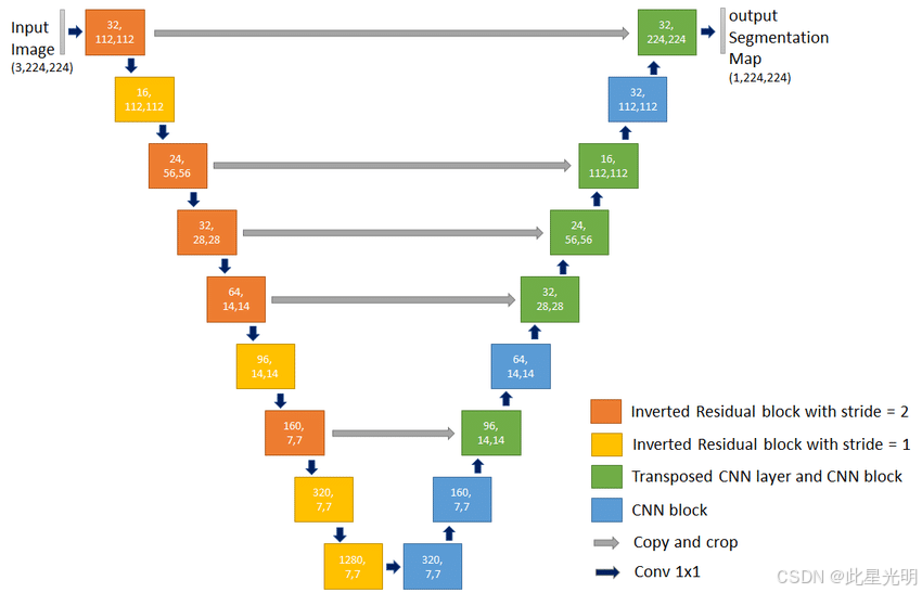
输出九个通道的原因是每个像素有九种可能的标签。可以将其视为多分类问题，其中每个像素被分类到九个类别中。
如前所述，编码器将是一个可选的预训练 MobileNetV2 模型，该模型已准备就绪，可在tf.keras.applications.中使用。编码器由模型中间层的特定输出组成。请注意，在训练过程中编码器不会进行训练，因为我们使用的是来自骨干特征提取模型的预训练权重。

base_model = tf.keras.applications.MobileNetV2(input_shape=[224, 224, 3], include_top=False)

# Use the activations of these layers
layer_names = [
    'block_1_expand_relu',
    'block_3_expand_relu',
    'block_6_expand_relu',
    'block_13_expand_relu',
    'block_16_project',
]
layers = [base_model.get_layer(name).output for name in layer_names]

# Create the feature extraction model
down_stack = tf.keras.Model(inputs=base_model.input, outputs=layers)

down_stack.trainable = False # Set this to False if using pre-trained weights

解码器/上采样器在 TensorFlow 示例中实现为一系列上采样块。参数为（过滤器数量，卷积核大小）。对于当前网络实现，3 的卷积核大小被认为是标准的（Sandler 等人，2018 年）。您可以增加或减少过滤器数量，但更多的过滤器意味着更多的参数和更长的训练时间。在 32 到 512 之间，每个连续的卷积层增加 2 倍，每个连续的转置卷积/上采样层减少，这在不同的卷积网络架构中非常常见。

up_stack = [
    pix2pix.upsample(512, 3),
    pix2pix.upsample(256, 3),
    pix2pix.upsample(128, 3),
    pix2pix.upsample(64, 3),
]
def unet_model(output_channels):
  inputs = tf.keras.layers.Input(shape=[224,224,3], name='first_layer')
  x = inputs

  # Downsampling through the model
  skips = down_stack(x)
  x = skips[-1]
  skips = reversed(skips[:-1])

  # Upsampling and establishing the skip connections
  for up, skip in zip(up_stack, skips):
    x = up(x)
    concat = tf.keras.layers.Concatenate()
    x = concat([x, skip])

  # This is the last layer of the model
  last = tf.keras.layers.Conv2DTranspose(
      output_channels, 3, strides=2, activation='softmax',
      padding='same', name='last_layer')

  x = last(x)

  return tf.keras.Model(inputs=inputs, outputs=x)

训练模型

现在，剩下的就是编译和训练模型了。这里使用的损失函数是 SparseCategoricalFocalLoss(from_logits=True)。使用这个损失函数的原因是 1) 因为网络试图为每个像素分配标签，就像多分类预测一样，2) 因为 focal loss 通过数据集中的分布来加权每个类别的相对贡献，以强调代表性不足的类别并抑制代表性过度的类别。在真实的分割掩码中，每个像素的值在 0-10 之间。这里的网络输出十个通道。本质上，每个通道都在尝试学习预测一个类别，而 SparseCategoricalFocalLoss(from_logits=True)是这种情况下的推荐损失函数。使用网络的输出，分配给像素的标签是值最高的通道。这就是 create_mask 函数所做的事情。

model = unet_model(OUTPUT_CHANNELS)

检查网络层输出形状

for layer in model.layers:
    print(layer.name, layer.output_shape)

为解决类别不平衡问题，找到用于 focal loss 函数的类别权重。

train_df = gpd.read_file('dlr_fusion_competition_germany_train_labels/dlr_fusion_competition_germany_train_labels_33N_18E_242N/labels.geojson')
inv_freq = np.array(1/(train_df.crop_id.value_counts()/len(train_df)))
inv_freq = [0.,*inv_freq]
class_weights = {0 : inv_freq[0], 1: inv_freq[1], 2: inv_freq[2], 3: inv_freq[3],
                4: inv_freq[4], 5: inv_freq[5], 6: inv_freq[6],
                7: inv_freq[7], 8: inv_freq[8], 9: inv_freq[9]}

def NormalizeData(data):
    return (data - np.min(data)) / (np.max(data) - np.min(data))

class_weights_list = list(class_weights.values())
print("class weights: ", class_weights_list)
scaled_class_weights = NormalizeData(class_weights_list)
scaled_class_weights_list = scaled_class_weights.tolist()
print("scaled class weights: ", scaled_class_weights_list)

在 SparseCategoricalFocalLoss 函数中，gamma 是聚焦参数。gamma 值越高，主要或“容易分类”的样本对损失的贡献相对于罕见或“难以分类”的样本就越小。gamma 的值必须是非负的，该损失函数的作者通过经验发现 gamma 值为 2 效果最佳（Lin 等人，2017 年）。你可以通过将类别权重作为参数添加到 SparseCategoricalFocalLoss 中来进行实验，例如 SparseCategoricalFocalLoss(gamma=2, class_weight=scaled_class_weights_list, from_logits=True) 。

我们将通过每个像素的准确率来衡量模型在训练过程中的性能。

model.compile(optimizer=tf.keras.optimizers.Adam(learning_rate=0.00001),
              loss=SparseCategoricalFocalLoss(gamma=2, from_logits=False), #tf.keras.losses.SparseCategoricalCrossentropy(from_logits=True),
              metrics=['accuracy', iou_score])

让我们尝试使用未训练/预训练模型，看看它在训练之前会做出什么预测。

def create_mask(pred_mask):
  pred_mask = tf.argmax(pred_mask, axis=-1)
  pred_mask = pred_mask[..., tf.newaxis]
  return pred_mask[0]
def show_predictions(image=None, mask=None, dataset=None, num=1):
  if image is None and dataset is None:
    # this is just for showing keras callback output. in practice this should be broken out into a different function
    sample_image = skio.imread(f'{img_dir}/tile_dlr_fusion_competition_germany_train_source_planet_5day_33N_18E_242N_2018_05_28_811.png') * (1/255.)
    sample_mask = skio.imread(f'{label_dir}/tile_dlr_fusion_competition_germany_train_source_planet_5day_33N_18E_242N_2018_05_28_811.png')
    mp = create_mask(model.predict(sample_image[tf.newaxis, ...]))
    mpe = tf.keras.backend.eval(mp)
    display([sample_image, sample_mask[..., tf.newaxis], mpe])
  elif dataset:
    for image, mask in dataset.take(num):
      pred_mask = model.predict(image)
      display([image[0], mask[0], create_mask(pred_mask)])
  else:
    mp = create_mask(model.predict(image[tf.newaxis, ...]))
    mpe = tf.keras.backend.eval(mp)
    display([image, mask, mpe])
show_predictions(image=sample_image, mask=sample_mask)

让我们观察模型在训练过程中的改进情况。为此，定义了一个回调函数，用于在每个训练周期后绘制测试图像及其预测掩码。

class DisplayCallback(tf.keras.callbacks.Callback):
  def on_epoch_end(self, epoch, logs=None):
    clear_output(wait=True)
    show_predictions()
    print ('\nSample Prediction after epoch {}\n'.format(epoch+1))

我们可能希望在 TensorBoard 中查看模型图和训练进度，因此我们将建立一个回调来将日志保存到一个专用目录，该目录将作为 TensorBoard 界面的接口。

# Load the TensorBoard notebook extension
%load_ext tensorboard
log_dir = os.path.join(user_outputs_dir,'logs/')
log_fit_dir = os.path.join(user_outputs_dir,'logs', 'fit')
log_fit_session_dir = os.path.join(user_outputs_dir,'logs', 'fit', datetime.datetime.now().strftime("%Y%m%d-%H%M%S"))
visualizations_dir = os.path.join(user_outputs_dir,'logs', 'vizualizations')
visualizations_session_dir = os.path.join(user_outputs_dir,'logs', 'vizualizations', datetime.datetime.now().strftime("%Y%m%d-%H%M%S"))

dirs = [log_fit_dir, visualizations_dir]
for dir in dirs:
  if (os.path.isdir(dir)):
    print("Making fresh log dir.")
    shutil.rmtree(dir)
  else:
    print("Fresh log dir exists.")

dirs = [log_dir, log_fit_dir, log_fit_session_dir, visualizations_dir, visualizations_session_dir]
for dir in dirs:
  if (not os.path.isdir(dir)):
    os.mkdir(dir)

tensorboard_callback = tf.keras.callbacks.TensorBoard(log_dir=log_fit_session_dir, histogram_freq=1, write_graph=True)

我们也可以使用 tf-explain 在 TensorBoard 中查看层激活情况，因此我们将建立一个回调来将激活可视化保存到一个专用目录，该目录将用于 TensorBoard 界面。

# get a batch of validation samples to plot activations for
for example in val_ds.take(1):
  image_val, label_val = example[0], example[1]
callbacks = [
    ActivationsVisualizationCallback(
        validation_data=(image_val, label_val),
        layers_name=["last_layer"],
        output_dir=visualizations_session_dir,
    ),
    DisplayCallback(),
    tensorboard_callback
]

拟合和查看

现在我们将实际训练模型 4 个周期（完整遍历训练数据集），并在每个周期后可视化验证图像上的预测结果。在实践中，您需要训练模型直到验证损失开始增加（这是过拟合的明显迹象）。根据这个数据集的经验，收敛大约发生在 50 个周期。我们将其减少到 4 个周期纯粹是为了快速演示目的。作为预览，在 50 个周期时，您应该观察到类似于以下的测试预测：

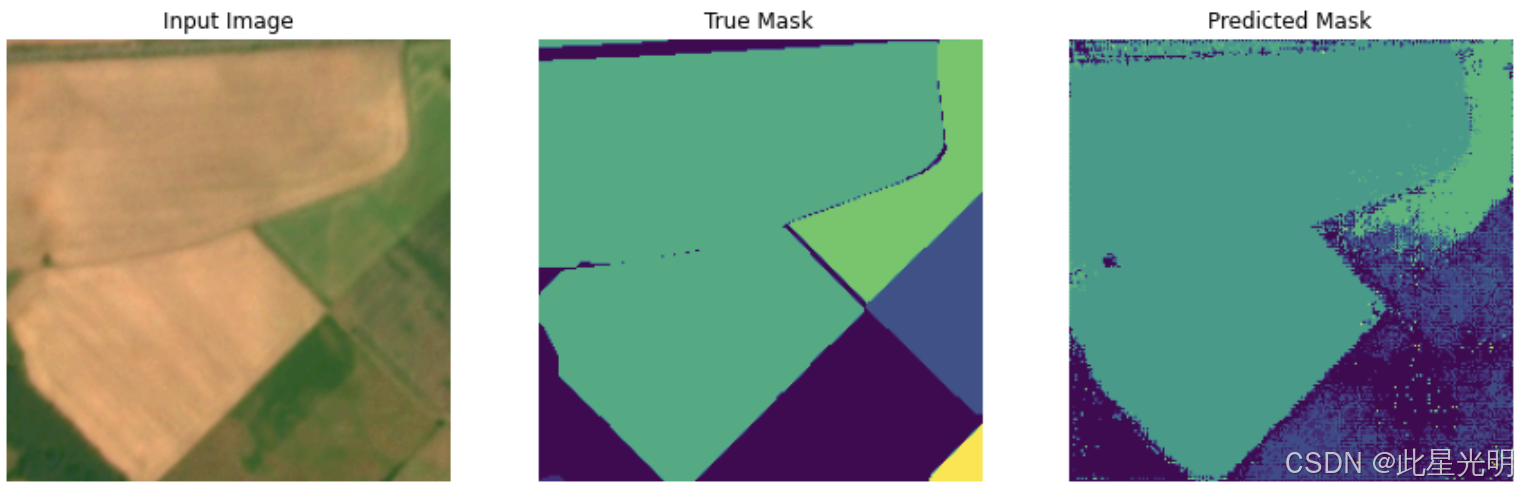
如果在 4 个周期后看到空白预测，请不要惊慌。

EPOCHS = 4

model_history = model.fit(train_ds,
                   steps_per_epoch=int(np.ceil(num_train_examples / float(batch_size))),
                   epochs=EPOCHS,
                   validation_data=val_ds,
                   validation_steps=int(np.ceil(num_val_examples / float(batch_size))),
                   callbacks=callbacks)

绘制模型随时间变化的学习曲线。

loss = model_history.history['loss']
val_loss = model_history.history['val_loss']

epochs = range(EPOCHS)

plt.figure()
plt.plot(epochs, loss, 'r', label='Training loss')
plt.plot(epochs, val_loss, 'bo', label='Validation loss')
plt.title('Training and Validation Loss')
plt.xlabel('Epoch')
plt.ylabel('Loss Value')
plt.ylim([0, 1])
plt.legend()
plt.show()

启动 TensorBoard

您在下方命令中将 logdir 设置为 …logs/visualizations 以查看激活值，或将 …logs/fit 设置为查看模型标量、图表、分布和直方图（如下所述）。

仪表板可以从顶部导航栏的选项卡中选择。

标量仪表板显示了损失和指标随每个训练周期的变化情况。您也可以使用它来跟踪训练速度、学习率和其他标量值。

图表仪表板帮助您可视化模型。在这种情况下，显示了 Keras 层的图，这可以帮助您确保模型构建正确。

分布和直方图仪表板显示了张量随时间的分布情况。这有助于可视化权重和偏差，并验证它们是否按预期方式变化。

%tensorboard --logdir "$visualizations_dir"

将模型保存到文件

我们将最终模型权重导出到您自己的谷歌驱动文件夹中。

if (not os.path.isdir(user_outputs_dir)):
  os.mkdir(user_outputs_dir)
save_model_path = os.path.join(user_outputs_dir,'model_out_batch_{}_ep{}_nopretrain_focalloss/'.format(batch_size, EPOCHS))
if (not os.path.isdir(save_model_path)):
  os.mkdir(save_model_path)
model.save(save_model_path)

进行预测

让我们做一些预测。为了节省时间，epoch 的数量保持较小，但你可以将其设置得更高以获得更准确的结果。我们将从可读的 workshop 目录中加载，以防你无法保存自己的模型。

# Optional, you can load the model from the saved version
load_from_checkpoint = True
if load_from_checkpoint == True:
  save_model_path = os.path.join(user_outputs_dir,'model_out_batch_{}_ep{}_nopretrain_focalloss/'.format(batch_size, EPOCHS))
  model = tf.keras.models.load_model(save_model_path, custom_objects={"loss": SparseCategoricalFocalLoss, "iou_score": iou_score})
else:
  print("inferencing from in memory model")

def get_predictions(image= None, dataset=None, num=1):
  if image is None and dataset is None:
    return ValueError("At least one of image or dataset must not be None.")
  if dataset:
    for image, mask in dataset.take(num):
      pred_mask = model.predict(image)
      return pred_mask
  else:
    pred_mask = create_mask(model.predict(image[tf.newaxis, ...]))
    pred_mask = tf.keras.backend.eval(pred_mask)
    return pred_mask

单张图像示例

display_num = 1
r_choices = np.random.choice(num_foreground_examples, 1)
for i in range(0, display_num * 2, 2):
  img_num = r_choices[i // 2]

temp_ds = get_baseline_dataset(foreground_list_x[img_num:img_num+1],
                               foreground_list_y[img_num:img_num+1],
                               preproc_fn=test_preprocessing_fn,
                               batch_size=1,
                               shuffle=False)

# Let's examine some of these augmented images

iterator = iter(temp_ds)
next_element = iterator.get_next()

batch_of_imgs, label = next_element

# Running next element in our graph will produce a batch of images

sample_image, sample_mask = batch_of_imgs[0], label[0,:,:,:]

# run and plot predicitions
pred_mask = get_predictions(sample_image)

show_predictions(image=sample_image, mask=sample_mask)

多图像示例

tiled_prediction_dir = os.path.join(user_outputs_dir,'predictions_test_focal_loss/')
if not os.path.exists(tiled_prediction_dir):
    os.makedirs(tiled_prediction_dir)

pred_masks = []
pred_paths = []
true_masks = []

for i in range(0, len(x_test_filenames)):
    img_num = i

    try:
      temp_ds = get_baseline_dataset(x_test_filenames[img_num:img_num+1],
                                   y_test_filenames[img_num:img_num+1],
                                   preproc_fn=test_preprocessing_fn,
                                   batch_size=1,
                                   shuffle=False)
    except Exception as e:
      print(str(e))

    # Let's examine some of these augmented images

    iterator = iter(temp_ds)
    next_element = iterator.get_next()

    batch_of_imgs, label = next_element

    # Running next element in our graph will produce a batch of images
    image, mask = batch_of_imgs[0], label[0,:,:,:]
    mask_int = tf.dtypes.cast(mask, tf.int32)
    true_masks.append(mask_int)
    print(y_test_filenames[img_num:img_num+1])
    print(np.unique(mask_int))

    # run and plot predicitions, only showing every 27th prediction
    #if img_num % 27 == 0:
    #    show_predictions(image=image, mask=mask)
    show_predictions(image=image, mask=mask)
    pred_mask = get_predictions(image)
    pred_masks.append(pred_mask)

    # save prediction images to file

    filename_split = os.path.splitext(x_test_filenames[img_num])
    filename_zero, fileext = filename_split
    basename = os.path.basename(filename_zero)
    pred_path = os.path.join(tiled_prediction_dir, "{}.png".format(basename))
    pred_paths.append(pred_path)
    tf.keras.preprocessing.image.save_img(pred_path,pred_mask, scale=False) # scaling is good to do to cut down on file size, but adds an extra dtype conversion step.

最后，我们将保存一个包含测试文件路径的 csv 文件，以便在下一课中轻松加载预测结果和标签，从而计算我们的评估指标。

path_df = pd.DataFrame(list(zip(x_test_filenames, y_test_filenames, pred_paths)), columns=["img_names", "label_names", "pred_names"])
path_df.to_csv(os.path.join(user_outputs_dir, "test_file_paths.csv"))

path_df = pd.DataFrame(list(zip(x_train_filenames, y_train_filenames)), columns=["img_names", "label_names"])
path_df.to_csv(os.path.join(user_outputs_dir, "train_file_paths.csv"))

path_df = pd.DataFrame(list(zip(x_val_filenames, y_val_filenames)), columns=["img_names", "label_names"])
path_df.to_csv(os.path.join(user_outputs_dir, "validate_file_paths.csv"))