PyTorch是一个开源的Python机器学习库，基于Torch库（一个有大量机器学习算法支持的科学计

算框架，有着与Numpy类似的张量（Tensor）操作，采用的编程语言是 Lua），底层由C++实现，

应用于人工智能领域，如计算机视觉和自然语言处理。

PyTorch官网：https://pytorch.org/，安装教程见主页。

通过 PyTorch 训练一个模型一般分为以下 4 个步骤：

准备数据 → 构建模型 → 定义损失函数与优化器 → 模型训练

一、张量创建

1、基本张量创建

1.1、torch.tensor(data)创建指定内容的张量

传入一个标量

import torch
tensor1 = torch.tensor(10)
print(tensor1)

tensor(10)

传入一个向量

tensor2 = torch.tensor([1,2,3])
print(tensor2)

# print(tensor2)

1.2、torch.Tensor(size)创建指定形状的张量

这个大写的Tensor也可以传入内容创建，默认是按形状

tensor3 = torch.Tensor(3,2,4)
print(tensor3)
print(tensor3.size())
print(tensor3.dtype)
result：
tensor([[[0., 0., 0., 0.],
         [0., 0., 0., 0.]],

        [[0., 0., 0., 0.],
         [0., 0., 0., 0.]],

        [[0., 0., 0., 0.],
         [0., 0., 0., 0.]]])
torch.Size([3, 2, 4])
torch.float32

1.3、torch.IntTensor()、torch.FloatTensor()等，或者torch.tensor中通过dtype指定参数类型创建指定类型的张量

tensor1 = torch.tensor([1,2,3],dtype = torch.int64)
print(tensor1)
print(tensor1.dtype)
tensor2 = torch.IntTensor([1,2,3])
print(tensor2)
print(tensor2.dtype)

result:tensor([1, 2, 3])
torch.int64
tensor([1, 2, 3], dtype=torch.int32)
torch.int32

2、指定区间的张量创建

2.1、torch.arange(start,end,step)在区间内按步长创建张量，不包括end

tensor1 = torch.arange(10,30,2)
print(tensor1)
print(tensor1.size())

tensor([10, 12, 14, 16, 18, 20, 22, 24, 26, 28])
torch.Size([10])

2.2、torch.linspace(start,end,steps)在区间内按元素数量创建张量，包括end

tensor1 = torch.linspace(10,30,5)
print(tensor1)
print(tensor1.size())

tensor([10., 15., 20., 25., 30.])
torch.Size([5])

2.3、torch.logspace(start,end,steps,base)在指数区间内按指定底数创建张量，包括end

tensor1 = torch.logspace(1,3,3,2)
print(tensor1)

tensor([2., 4., 8.])

3、按数值填充张量

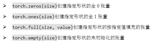
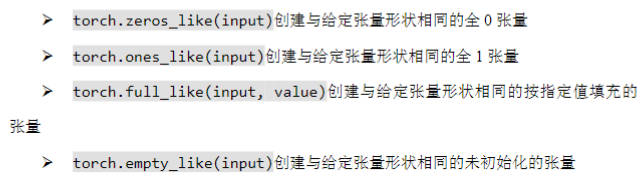
补充：torch.eye创建单位矩阵，如果只传入一个值那就是方阵

tensor1 = torch.eye(3,4)
print(tensor1)

tensor([[1., 0., 0., 0.],
        [0., 1., 0., 0.],
        [0., 0., 1., 0.]])

4、随机张量创建

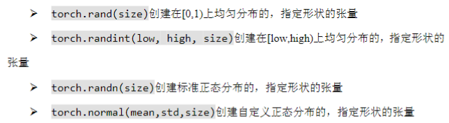
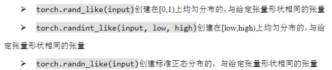
补充：torch.randperm(n)生成0到n-1的随机排列，类似洗牌

tensor1 = torch.randperm(6)
print(tensor1)

tensor([5, 2, 0, 1, 4, 3])

torch.random.initial_seed()查看随机数种子

torch.manual_seed(seed)设置随机数种子

print(torch.random.initial_seed())
#1381529020242300
torch.manual_seed(42)
print(torch.random.initial_seed())
#42

二、张量转换

1、张量元素类型转换

1.1、Tensor.type(dtype)修改张量类型

import torch
tensor1 = torch.tensor([1,2,3])
print(tensor1,tensor1.dtype)
tensor1 = tensor1.type(torch.float32)
print(tensor1,tensor1.dtype)

tensor([1, 2, 3]) torch.int64
tensor([1., 2., 3.]) torch.float32

1.2、Tensor.double()等修改张量的类型

tensor1 = tensor1.double()
print(tensor1,tensor1.dtype)

tensor([1., 2., 3.], dtype=torch.float64) torch.float64

补充：torch.complex是复数类型

2、Tensor与ndarray转换

注意copy()是对于ndarray而言的，写代码的时候要看清楚类型，在ndarray的后面接一个copy()，

对于tensor也有一个方法叫clone()

2.1、Tensor.numpy()将Tensor转换为ndarray，共享内存，使用copy()避免共享内存

这里可以看出共享内存

np.set_printoptions(precision = 6)
torch.set_printoptions(precision = 6)
tensor1 = torch.rand(3,2)
print(tensor1)
ndarray1 = tensor1.numpy()
print(ndarray1)
ndarray1[1,0] = 2
print(ndarray1)
print(tensor1)

tensor([[0.306238, 0.535756],
        [0.378546, 0.316012],
        [0.790295, 0.365583]])
[[0.306238 0.535756]
 [0.378546 0.316012]
 [0.790295 0.365583]]
[[0.306238 0.535756]
 [2.       0.316012]
 [0.790295 0.365583]]
tensor([[0.306238, 0.535756],
        [2.000000, 0.316012],
        [0.790295, 0.365583]])

使用copy()不共享内存

ndarray2 = tensor1.numpy().copy()
tensor1[:,0] = 10
print(tensor1)
print(ndarray2)

tensor([[10.000000,  0.049914],
        [10.000000,  0.325573],
        [10.000000,  0.058194]])
[[0.043996 0.049914]
 [2.       0.325573]
 [0.902513 0.058194]]

2.2、torch.from_numpy(ndarray)将ndarray转换为Tensor，共享内存，使用copy避免内存共享

ndarray1 = np.random.randn(3)
tensor1 = torch.from_numpy(ndarray1)
print(tensor1)
print(ndarray1)

tensor([-0.985477,  0.635086,  1.754846], dtype=torch.float64)
[-0.985477  0.635086  1.754846]

tensor2 = torch.from_numpy(ndarray1.copy())
tensor2[0] = 1.5
print(tensor2)
print(ndarray1)

tensor([1.500000, 1.199748, 1.003381], dtype=torch.float64)
[-0.62402   1.199748  1.003381]

3、Tensor与标量转换

若张量中只有一个元素，Tensor.item()可以提取张量中元素为标量

tensor1 = torch.tensor(10)
print(tensor1)
print(tensor1.shape)
a = tensor1.item()
print(a)

tensor(10)
torch.Size([])
10

三、张量数值计算

1、基本运算

1.1、四则运算

下划线会修改原数据

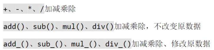
print(tensor1.add(10))
print(tensor1)

tensor([[14, 11, 13],
        [19, 14, 16]])
tensor([[4, 1, 3],
        [9, 4, 6]])

print(tensor1.add_(10))
print(tensor1)

tensor([[14, 11, 13],
        [19, 14, 16]])
tensor([[14, 11, 13],
        [19, 14, 16]])

1.2、取负数neg()、neg_()

同样，加下划线改变原数据

1.3、求幂**、pow()、pow_()

对每个元素求幂，同样，加下划线改变原数据

1.4、求平方根sqrt()、sqrt_()

同上

1.5、exp()、exp_()以e为底数求幂

同上

1.6、log()、log_()以 e 为底求对数

同上

2、哈达玛积（元素级乘法）

两个矩阵对应位置元素相乘称为哈达玛积（Hadamard product），使用*、mul()实现两个形状相同

的张量之间对位相乘。

3、矩阵乘法运算@、matmul()、mm()

mm()严格用于二维矩阵相乘。@、matmul()支持多维张量，按最后两个维度做矩阵乘法，其他维

度相同，或者至少一个张量对应维度为 1，广播后进行运算，像这样。

tensor1 = torch.Tensor(4,2,3,5)
tensor2 = torch.Tensor(1,1,5,6)
print((tensor1 @ tensor2).shape)

意思就是张量相乘，维度必须一样，然后最后两个维度要符合矩阵乘法的规格。

tensor1 = torch.tensor([[1,2],[3,4],[0,1]])
tensor2 = torch.tensor([[5,6],[7,8]])
print(tensor1 @ tensor2)

tensor([[19, 22],
        [43, 50],
        [ 7,  8]])

4、节省内存

首先我们讲哈达玛积，如果直接运行print(X*Y)，这样X的值本身不会改变；如果X = X * Y，做了一

步这样的赋值操作，其实是创建了一个新的变量，只是这个变量名字叫X而已，没有做到节省内存

空间的作用，可以查看id，如果运行的是mul_，则可以保存，如果用X *= Y，这样也可以。

X = torch.randint(1,10,(3,2,4))
Y = torch.randint(1,10,(3,2,4))
print(id(X))
X = X * Y
print(id(X))

2486393500000
2486393499120

接下来讲矩阵乘法，矩阵乘法用X @= Y这样的形式行不通，得X[:] = X @ Y，用 X @ Y 的结果，

原地覆盖 X 本身的所有元素，这样能节省内存的前提是，乘出来的矩阵规格要小于等于之前的规

格并且能广播，广播也有batch广播和矩阵规格广播，广播需要维度为1。

四、张量运算函数

这些都是多对一的函数，有一个统计聚合效果

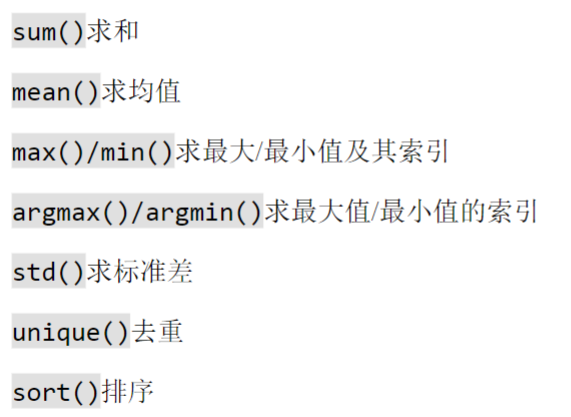
sum函数在用的时候可以设置dim，这个指的是针对哪一个维度，比如我这里的dim = 0，就是针对

batch = 3这个维度，设置哪一个dim，就是把那个dim压缩没

import torch
tensor1 = torch.randint(1,10,(3,2,4))
print(tensor1)
print(tensor1.sum())
sum = torch.sum(tensor1, dim=0)
print(sum)

tensor([[[2, 4, 5, 6],
         [6, 6, 5, 5]],

        [[1, 4, 9, 4],
         [8, 2, 2, 9]],

        [[6, 5, 4, 2],
         [8, 2, 2, 3]]])
tensor(110)
tensor([[ 9, 13, 18, 12],
        [22, 10,  9, 17]])

五、张量索引

1、简单索引

可以【0，1，2】也可以【0】【1】【2】这样写，然后如果写比如【0，1】，意思就是第一个矩

阵的第一行。

import torch
tensor1 = torch.randint(1,10,(3,5,4))
print(tensor1)
print(tensor1[0,1,2])

tensor([[[9, 2, 1, 1],
         [1, 6, 5, 9],
         [6, 1, 2, 4],
         [4, 3, 7, 5],
         [2, 4, 6, 2]],

        [[1, 5, 4, 7],
         [8, 9, 3, 7],
         [1, 1, 3, 1],
         [1, 2, 1, 7],
         [1, 7, 7, 7]],

        [[8, 3, 9, 1],
         [7, 9, 1, 3],
         [7, 2, 3, 2],
         [3, 7, 2, 8],
         [2, 5, 8, 6]]])
tensor(5)

2、范围索引

看这种范围索引主要要看逗号在哪里，注意：-1就是最后一行

这个意思是所有矩阵的第1行拼起来

print(tensor1[:,1])

tensor([[3, 6, 2, 2],
        [2, 6, 3, 7],
        [5, 3, 2, 4]])

这个意思是包括第1个矩阵的之后所有矩阵，每个矩阵的1到3行，这里也可以写1:4:2，考虑步长

print(tensor1[1:,1:4])

tensor([[[2, 6, 3, 7],
         [4, 1, 4, 9],
         [6, 6, 5, 8]],

        [[5, 3, 2, 4],
         [5, 2, 8, 3],
         [6, 9, 9, 9]]])

3、列表索引

这个就相当于【0，1，3】和【1，2，1】，列表索引的列表长度要一致

print(tensor1[[0,1],[1,2],[3,1]])

tensor([2, 1])

上面是一一对应的情况，以下是一对多的情况

print(tensor1[[[0],[1]],[1,2]])

tensor([[[3, 6, 2, 2],
         [3, 7, 6, 3]],

        [[2, 6, 3, 7],
         [4, 1, 4, 9]]])

4、布尔索引

mask = tensor1[:,0,2] > 4
print(mask)
print(tensor1[mask])

tensor([ True, False,  True])
tensor([[[4, 3, 7, 4],
         [3, 6, 2, 2],
         [3, 7, 6, 3],
         [3, 2, 3, 7],
         [8, 9, 8, 9]],

        [[7, 6, 5, 4],
         [5, 3, 2, 4],
         [5, 2, 8, 3],
         [6, 9, 9, 9],
         [9, 3, 3, 2]]])

mask的shape一定要和矩阵的shape保持一致，不然会报错，所以这里要提前转置一下

mask = tensor1[:,1,:] > 5
print(mask)
tensor2 = tensor1.mT
print(tensor2[mask])

tensor([[False,  True, False, False],
        [False,  True, False,  True],
        [False, False, False, False]])
tensor([[3, 6, 7, 2, 9],
        [1, 6, 1, 6, 8],
        [5, 7, 9, 8, 3]])

六、张量形状操作

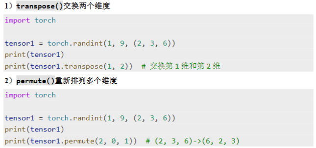
1、交换维度

如果是一般情况下，一个tensor.T做转置，是全部反转，比如【3，2，5】这个shape，T了之后就

是【5，2，3】，这样元素的坐标也是全部反转，如果只想转置矩阵，要用.mT，m是matrix的意

思。

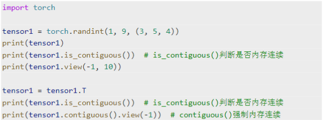
2、调整形状

 

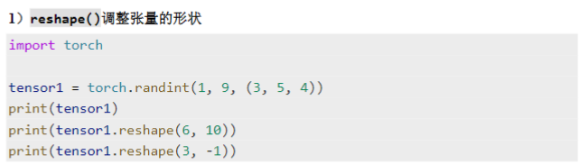
用reshape的时候，元素个数要匹配，-1就是自己计算维度，在这个案例中为20。

2）view()调整张量的形状，需要内存连续，共享内存

is_contiguous()判断是否连续，contiguous()转成连续

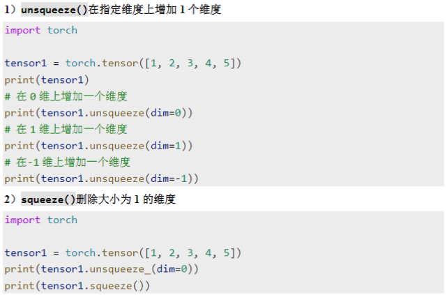
3、增删维度

在这里-1就是最后一维

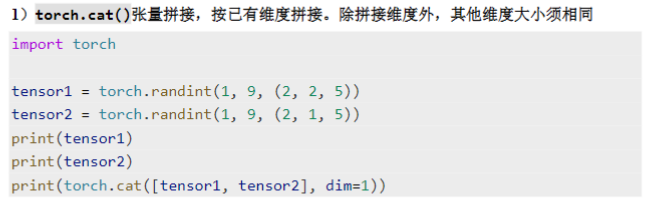
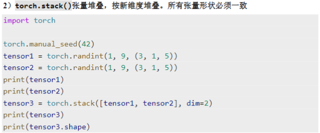
4、张量的拼接和堆叠

七、自动微分模块（计算梯度）

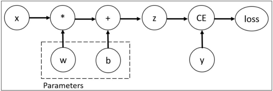
自动微分的关键就是记录节点的数据与运算。数据记录在张量的 data 属性中，计算记录在张量的

grad_fn 属性中。

x = torch.tensor(10.0)
y = torch.tensor(3.0)
w = torch.rand(1,1,requires_grad=True)
b = torch.rand(1,1,requires_grad=True)
z = w * x + b
print(z)
print(z.requires_grad)
print(x.is_leaf)
print(y.is_leaf)
print(z.is_leaf)
print(w.is_leaf)
print(b.is_leaf)
loss = torch.nn.MSELoss()
loss_value = loss(z,y)
print(loss_value)
print(loss_value.is_leaf)
loss_value.backward()
print(w.grad)
print(b.grad)

tensor([[4.8459]], grad_fn=<AddBackward0>)
True
True
True
False
True
True
tensor(3.4073, grad_fn=<MseLossBackward0>)
False
tensor([[36.9177]])
tensor([[3.6918]])

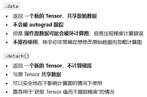
有时我们希望将某些计算移动到计算图之外，可以使用 Tensor.detach()返回一个新的变量，该变

量与原变量具有相同的值，但丢失计算图中如何计算原变量的信息。换句话说，梯度不会在该变量

处继续向下传播。

这里的z2不可以运行backward方法，因为requires_grad被关闭了

x = torch.tensor(2.0, requires_grad=True)
y = x.detach()
print(x)
print(y)
z1 = x ** 2
z1.backward()
print(x.grad)
print(z1)
z2 = y ** 2
print(z2)

tensor(2., requires_grad=True)
tensor(2.)
tensor(4.)
tensor(4., grad_fn=<PowBackward0>)
tensor(4.)

八、线性回归案例

import os
os.environ["KMP_DUPLICATE_LIB_OK"] = "TRUE"

import torch
import matplotlib.pyplot as plt
from torch import nn, optim
from torch.utils.data import TensorDataset, DataLoader

x = torch.randn(100,1)
w = torch.tensor([2.5])
b = torch.tensor([5.2])
noise = torch.randn(100,1) * 0.5
y = w * x + b + noise
dataset = TensorDataset(x, y)
dataloader = DataLoader(dataset,batch_size = 10,shuffle = True)
model = nn.Linear(1,1)
loss = nn.MSELoss()
optimizer = optim.SGD(model.parameters(),lr = 0.001)
epochs = 1000
loss_list = []
for epoch in range(epochs):
    total_loss = 0
    iter_num = 0
    for x_batch, y_batch in dataloader:
        y_pred = model(x_batch)
        loss_value = loss(y_pred, y_batch)
        loss_value.backward()
        optimizer.step()
        optimizer.zero_grad()

        total_loss += loss_value.item()
        iter_num += 1
    loss_list.append(total_loss / iter_num)
print("斜率：",model.weight)
print("截距：",model.bias)

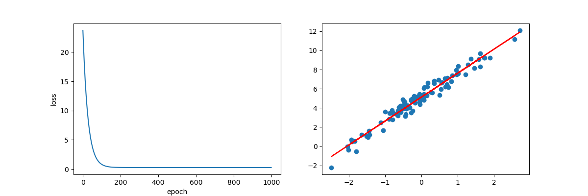
fig,ax = plt.subplots(1,2,figsize=(12,4))
ax[0].plot(loss_list)
ax[0].set_xlabel('epoch')
ax[0].set_ylabel('loss')
ax[1].scatter(x,y)
y_hat = model.weight.item() * x + model.bias.item()
ax[1].plot(x,y_hat,color='red')
plt.show()

E:\anaconda3\envs\PyTorch\python.exe E:\Py_project\PyTorch\linear_regression.py 
斜率： Parameter containing:
tensor([[2.4992]], requires_grad=True)
截距： Parameter containing:
tensor([5.1325], requires_grad=True)

九、激活函数

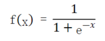
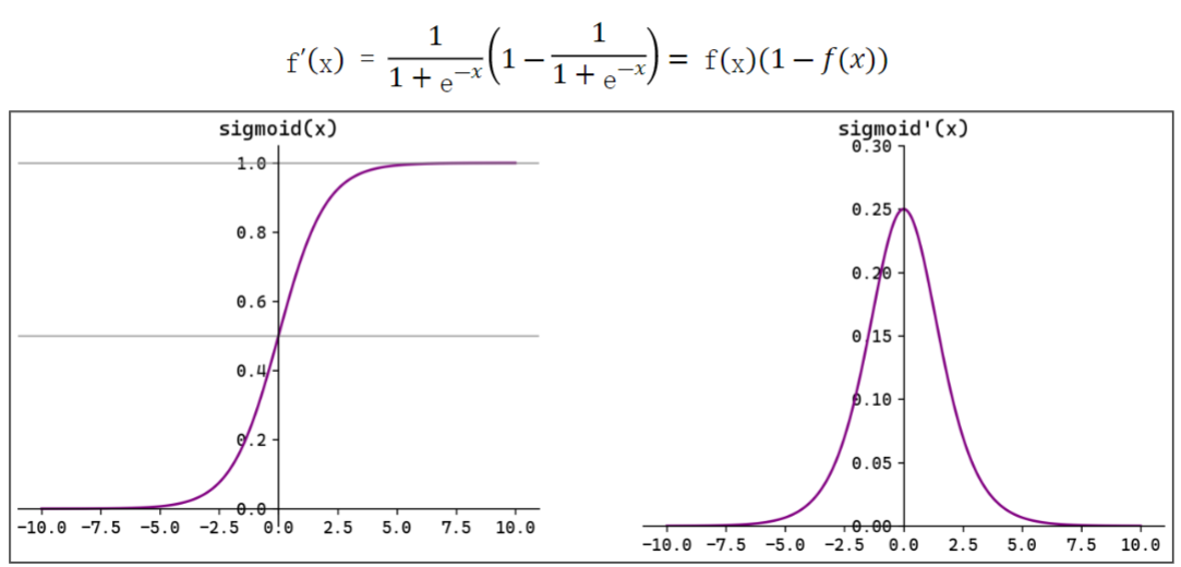
1、Sigmoid

import os
os.environ["KMP_DUPLICATE_LIB_OK"] = "TRUE"
import torch
import matplotlib.pyplot as plt

x = torch.linspace(-10,10,1000,requires_grad=True)
y = torch.sigmoid(x)

fig,ax = plt.subplots(1,2,figsize=(12,4))
ax[0].plot(x.data,y.data,color='purple')
ax[0].set_title('sigmoid(x)')
ax[0].axhline(y = 1,color='gray',linewidth = 1,alpha = 0.7)
ax[0].axhline(y = 0.5,color='gray',linewidth = 1,alpha = 0.7)
ax[0].spines['top'].set_visible(False)
ax[0].spines['right'].set_visible(False)
ax[0].spines['left'].set_position('zero')
ax[0].spines['bottom'].set_position('zero')

y.sum().backward()

ax[1].plot(x.data,x.grad,color='purple')
ax[1].set_title("sigmoid'(x)")
ax[1].spines['top'].set_visible(False)
ax[1].spines['right'].set_visible(False)
ax[1].spines['left'].set_position('zero')
ax[1].spines['bottom'].set_position('zero')
plt.show()

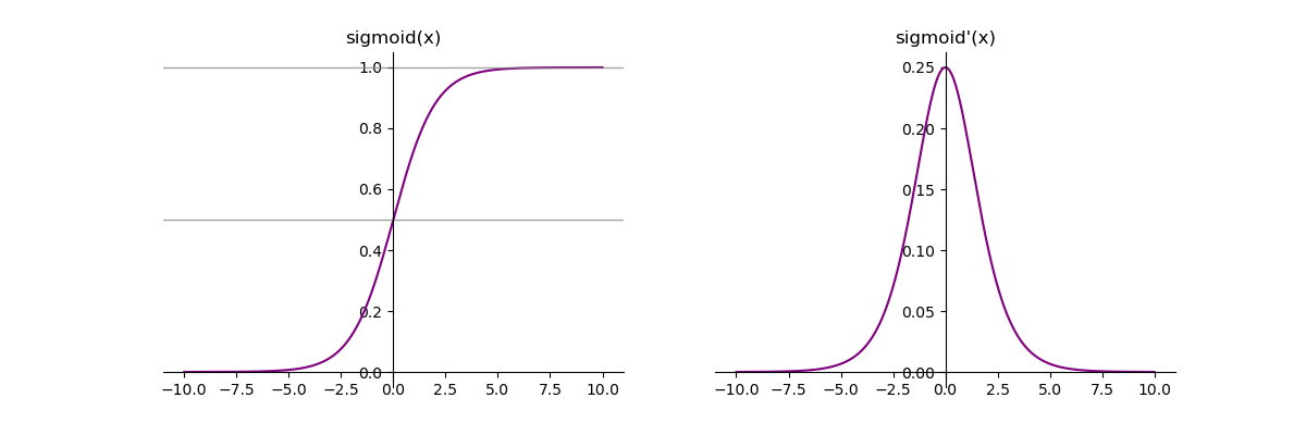
 注意这里为什么要

y.sum().backward()

因为backward只能对标量使用，如果直接对y进行backward就不知道到底要对哪一个数值进行求梯

度，为什么要选择sum而不是拆开来对应x1y1这样求呢，是因为能影响到梯度的只有对应的yn，其

它的是当作常数，所以即使sum了也不影响，如下图：

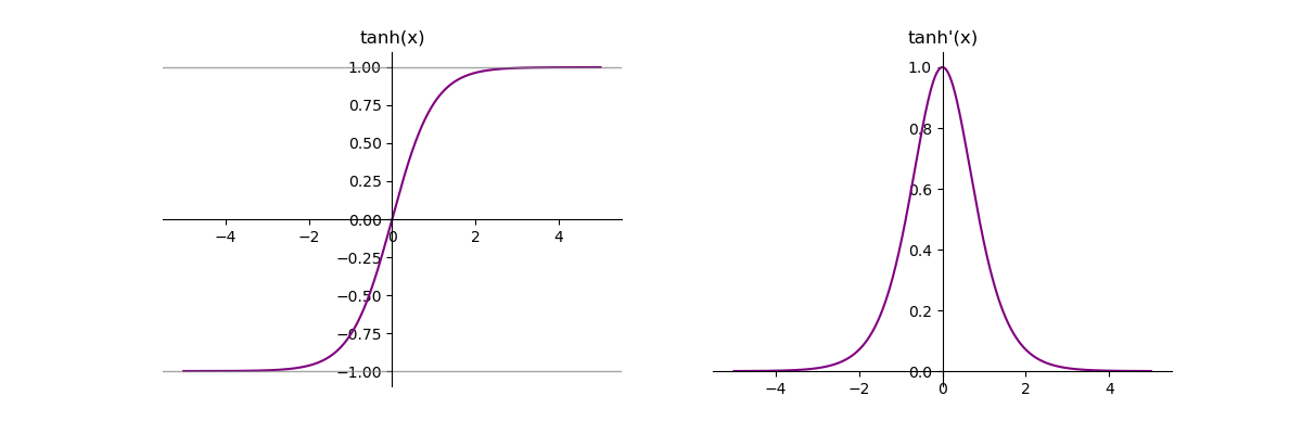
2、Tanh

import os
os.environ["KMP_DUPLICATE_LIB_OK"] = "TRUE"
import torch
import matplotlib.pyplot as plt

x = torch.linspace(-5,5,1000,requires_grad=True)
y = torch.tanh(x)

fig,ax = plt.subplots(1,2,figsize=(12,4))
ax[0].plot(x.data,y.data,color='purple')
ax[0].set_title('tanh(x)')
ax[0].axhline(y = 1,color='gray',linewidth = 1,alpha = 0.7)
ax[0].axhline(y = -1,color='gray',linewidth = 1,alpha = 0.7)
ax[0].spines['top'].set_visible(False)
ax[0].spines['right'].set_visible(False)
ax[0].spines['left'].set_position('zero')
ax[0].spines['bottom'].set_position('zero')

y.sum().backward()

ax[1].plot(x.data,x.grad,color='purple')
ax[1].set_title("tanh'(x)")
ax[1].spines['top'].set_visible(False)
ax[1].spines['right'].set_visible(False)
ax[1].spines['left'].set_position('zero')
ax[1].spines['bottom'].set_position('zero')
plt.show()

3、ReLU

import torch
import matplotlib.pyplot as plt

x = torch.linspace(-5,5,1000,requires_grad=True)
y = torch.relu(x)

fig,ax = plt.subplots(1,2,figsize=(12,4))
ax[0].plot(x.data,y.data,color='purple')
ax[0].set_title('relu(x)')
ax[0].spines['top'].set_visible(False)
ax[0].spines['right'].set_visible(False)
ax[0].spines['left'].set_position('zero')
ax[0].spines['bottom'].set_position('zero')

y.sum().backward()

ax[1].plot(x.data,x.grad,color='purple')
ax[1].set_title("relu'(x)")
ax[1].spines['top'].set_visible(False)
ax[1].spines['right'].set_visible(False)
ax[1].spines['left'].set_position('zero')
ax[1].spines['bottom'].set_position('zero')
plt.show()

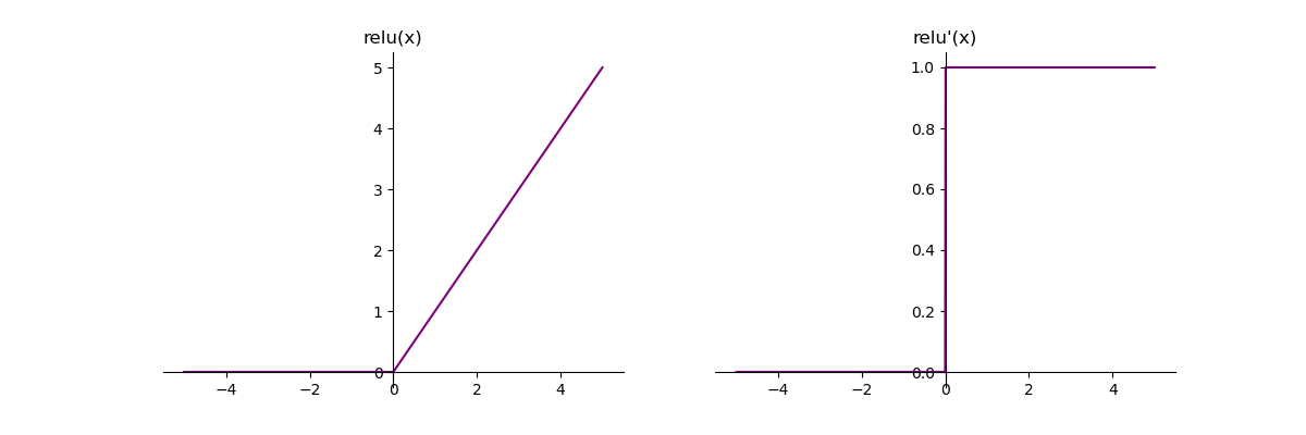
4、softmax

import torch
x = torch.randn(3,5)
y_prob = torch.softmax(x, dim=1)
print(y_prob)

tensor([[0.6430, 0.0900, 0.2124, 0.0300, 0.0246],
        [0.0299, 0.1759, 0.2867, 0.0711, 0.4363],
        [0.3348, 0.4210, 0.2128, 0.0076, 0.0238]])

十、全连接层（初始化）

1、常见初始化方法

初始化为全0

import torch.nn as nn
linear = nn.Linear(5, 2)
# 初始化全0
nn.init.zeros_(linear.bias)
print(linear.bias)

Parameter containing:
tensor([0., 0.], requires_grad=True)

初始化为任意常数用constant

import torch.nn as nn
linear = nn.Linear(5, 2)
nn.init.constant_(linear.bias,10)
print(linear.bias)

Parameter containing:
tensor([10., 10.], requires_grad=True)

秩初始化

import torch.nn as nn
linear = nn.Linear(5, 2)
nn.init.eye_(linear.weight)
print(linear.weight)

Parameter containing:
tensor([[1., 0., 0., 0., 0.],
        [0., 1., 0., 0., 0.]], requires_grad=True)

正态分布初始化

linear = nn.Linear(5, 2)
nn.init.normal_(linear.weight,mean = 5,std = 1)
print(linear.weight)

Parameter containing:
tensor([[4.0496, 3.6883, 5.0904, 5.5787, 4.6238],
        [6.3297, 6.1959, 4.6086, 5.1574, 6.2251]], requires_grad=True)

均匀分布初始化

linear = nn.Linear(5, 2)
nn.init.uniform_(linear.weight,0,10)
print(linear.weight)

Parameter containing:
tensor([[5.3156, 3.2887, 2.0559, 0.8858, 7.4100],
        [9.8123, 1.7759, 1.9474, 5.4194, 5.7101]], requires_grad=True)

2、Xavier初始化（Glorot初始化）

适用于sigmoid和Tanh等激活函数，能有效缓解梯度消失或爆炸问题

import torch.nn as nn
linear = nn.Linear(5, 2)
nn.init.xavier_normal_(linear.weight)
print(linear.weight)
nn.init.xavier_uniform_(linear.weight)
print(linear.weight)

Parameter containing:
tensor([[ 0.1092,  0.6596, -0.2596,  0.1790,  0.1906],
        [ 1.1577,  0.1663,  0.0516,  0.4451, -0.9941]], requires_grad=True)
Parameter containing:
tensor([[-0.3551, -0.0147, -0.5234,  0.4733,  0.1845],
        [ 0.0142,  0.1118, -0.7389,  0.9132,  0.6893]], requires_grad=True)

3、He初始化（Kaiming）

主要适用于ReLU及其变体

linear = nn.Linear(5, 2)
nn.init.kaiming_normal_(linear.weight)
print(linear.weight)
nn.init.kaiming_uniform_(linear.weight)
print(linear.weight)

Parameter containing:
tensor([[ 0.2884,  0.4597,  0.9206, -0.9007, -1.4727],
        [ 0.1024,  0.7552,  1.3354, -0.0632,  0.2416]], requires_grad=True)
Parameter containing:
tensor([[-0.2535,  0.0838, -1.0336, -0.2692, -0.2258],
        [ 0.2634, -0.4902,  0.8401, -0.4683,  0.1186]], requires_grad=True)

十一、正则化dropout

随机失活dropout

import torch
import torch.nn as nn

x = torch.randint(1,10,(10,),dtype=torch.float)
print(x)
dropout = nn.Dropout(p = 0.2)
y = dropout(x)
print(y)

tensor([1., 7., 1., 8., 7., 7., 5., 7., 3., 6.])
tensor([ 0.0000,  8.7500,  1.2500, 10.0000,  0.0000,  8.7500,  0.0000,  0.0000,
         3.7500,  7.5000])

十二、搭建神经网络

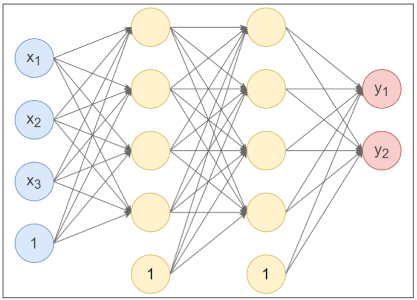
1、搭建神经网络

第 1 个隐藏层：使用 Xavier 正态分布初始化权重，激活函数使用 Tanh。

第 2 个隐藏层：使用 He 正态分布初始化权重，激活函数使用 ReLU。

输出层：按默认方式初始化，激活函数使用 Softmax。

import torch
import torch.nn as nn

class NN_model(nn.Module):
    def __init__(self):
        super().__init__()
        self.linear1 = nn.Linear(3, 4)
        nn.init.xavier_normal_(self.linear1.weight)
        self.linear2 = nn.Linear(4, 4)
        nn.init.kaiming_normal_(self.linear2.weight)
        self.out = nn.Linear(4, 2)
    def forward(self, x):
        x = self.linear1(x)
        x = torch.tanh(x)
        x = self.linear2(x)
        x = torch.relu(x)
        x = self.out(x)
        y = torch.softmax(x,dim = 1)
        return y

if __name__ == '__main__':
    x = torch.randn(10,3)
    model = NN_model()
    y_pred = model(x)
    print("预测输出分类概率：",y_pred)

预测输出分类概率： tensor([[0.5959, 0.4041],
        [0.3317, 0.6683],
        [0.1820, 0.8180],
        [0.5968, 0.4032],
        [0.5942, 0.4058],
        [0.5982, 0.4018],
        [0.5165, 0.4835],
        [0.6301, 0.3699],
        [0.4951, 0.5049],
        [0.5866, 0.4134]], grad_fn=<SoftmaxBackward0>)

2、查看模型参数

2.1、全部打出来

print(model.linear1.weight)
print(model.linear1.bias)
print(model.linear2.weight)
print(model.linear2.bias)
print(model.out.weight)
print(model.out.bias)

2.2、for循环查找，调用model.parameters，但是不知道名称

for param in model.parameters():
    print(param)

2.3、for循环，调用model.named_parameters

for name,param in model.named_parameters():
    print(name)
    print(param)

2.4、调用model.state_dict()查看参数字典

print(model.state_dict())

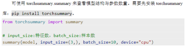
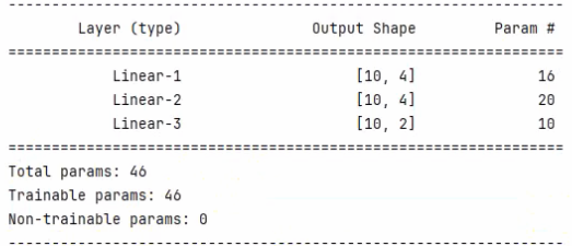
3、查看模型结构和参数数量

输出示例

 4、使用Sequential定义模型

可以通过 torch.nn.Sequential 来构建模型，将各层按顺序传入。

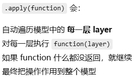
import os
os.environ["KMP_DUPLICATE_LIB_OK"] = "TRUE"
import torch
import torch.nn as nn
from torchsummary import summary

x = torch.randn(10,3)
model = nn.Sequential(
    nn.Linear(3,4),
    nn.Tanh(),
    nn.Linear(4,4),
    nn.ReLU(),
    nn.Linear(4,2),
    nn.Softmax(dim=1)
)

def init_params(layer):
    # 判断如果是线性层，就做参数初始化
    if isinstance(layer, nn.Linear):
        nn.init.xavier_uniform_(layer.weight)
        nn.init.constant_(layer.bias, 0.01)

model.apply(init_params)

y_pred = model(x)
print("预测输出：",y_pred)
summary(model,(3,),batch_size=10,device='cpu')

预测输出： tensor([[0.4771, 0.5229],
        [0.4563, 0.5437],
        [0.7329, 0.2671],
        [0.9581, 0.0419],
        [0.7896, 0.2104],
        [0.4530, 0.5470],
        [0.4521, 0.5479],
        [0.4652, 0.5348],
        [0.4403, 0.5597],
        [0.9639, 0.0361]], grad_fn=<SoftmaxBackward0>)
----------------------------------------------------------------
        Layer (type)               Output Shape         Param #
================================================================
            Linear-1                    [10, 4]              16
              Tanh-2                    [10, 4]               0
            Linear-3                    [10, 4]              20
              ReLU-4                    [10, 4]               0
            Linear-5                    [10, 2]              10
           Softmax-6                    [10, 2]               0
================================================================
Total params: 46
Trainable params: 46
Non-trainable params: 0
----------------------------------------------------------------
Input size (MB): 0.00
Forward/backward pass size (MB): 0.00
Params size (MB): 0.00
Estimated Total Size (MB): 0.00
----------------------------------------------------------------