线性回归

一元线性回归：

• 最优化问题（凸优化）
• 民主投票
• 距离的衡量

损失函数：

                 

使用Boston数据集实现一元线性回归（下载csv文件）

LinearRegression 要的是 二维特征矩阵，现在的 x_train 是 一维 Series，需要 reshape 成 (n_samples, 1)

import numpy as np
from sklearn import datasets
import matplotlib.pyplot as plt

import pandas as pd
boston = pd.read_csv('./BostonHousing.csv')
x = boston.rm
y = boston.medv
x = x[y<50]
y = y[y<50]
from sklearn.model_selection import train_test_split
x_train,x_test,y_train,y_test=train_test_split(x,y,train_size=0.7,random_state=233)

plt.scatter(x_train,y_train)
plt.show()

# 自定义方法：公式实现
def fit(x,y):
    a_up = np.sum((x-np.mean(x))*(y-np.mean(y)))
    a_bottom = np.sum((x-np.mean(x))**2)
    a = a_up/a_bottom
    b = np.mean(y)-a*np.mean(x)
    return a,b

a,b = fit(x_train,y_train)
plt.scatter(x_test,y_test)
plt.scatter(x_test,a*x_test+b,c='r')
plt.show()

sklearn实现一元线性回归

问题：线性回归默认不能直接处理 NaN

解决方法：用中位数填充缺失值

from sklearn.linear_model import LinearRegression
lin_reg = LinearRegression()
# 缺失值处理
fill_value = x_train.median()

x_train = x_train.fillna(fill_value)
x_test  = x_test.fillna(fill_value)
# 使用fit方法当存在nan值时会报错ValueError: Input X contains NaN.
lin_reg.fit(x_train.values.reshape(-1,1),y_train)
y_predict = lin_reg.predict(x_test.values.reshape(-1,1))
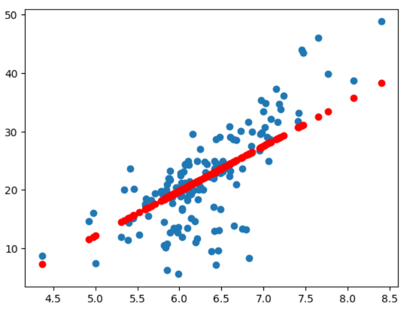
plt.scatter(x_test,y_test)
plt.scatter(x_test,y_predict,c='r')
plt.show()

多元线性回归：

找参数最小化目标函数：

sklearn实现多元线性回归

直接将读取的数据转化为numpy的二维数组格式，并使用中位数填充缺失值

# sklearn 接收的是 NumPy 的二维数组（ndarray）
# Pandas 的 Series / DataFrame 要 显式转成 .values 或 .to_numpy()
boston_data = boston.to_numpy()
x = boston_data[:,:-1]
y = boston_data[:,-1]
x = x[y<50]
y = y[y<50]
x_train,x_test,y_train,y_test=train_test_split(x,y,train_size=0.7,random_state=233)
# 缺失值处理
from sklearn.impute import SimpleImputer

imputer = SimpleImputer(strategy="median")
imputer.fit(x_train) 
x_train = imputer.transform(x_train)
x_test  = imputer.transform(x_test)
lin_reg.fit(x_train,y_train)
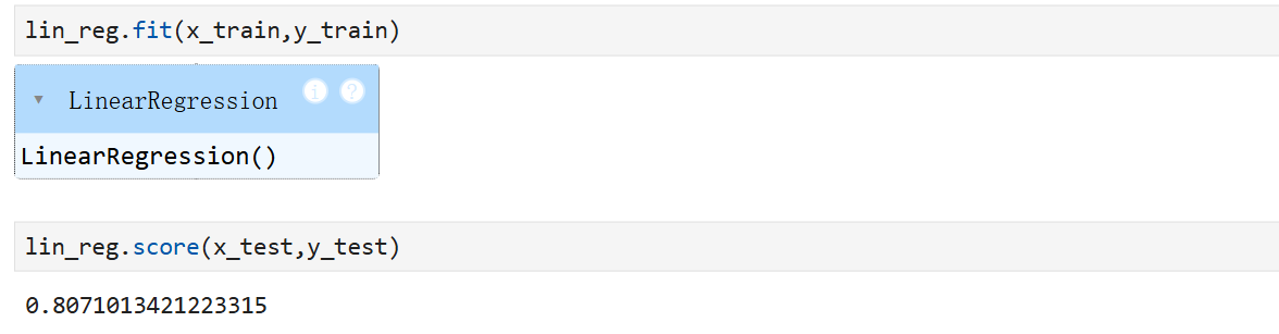
lin_reg.score(x_test,y_test)

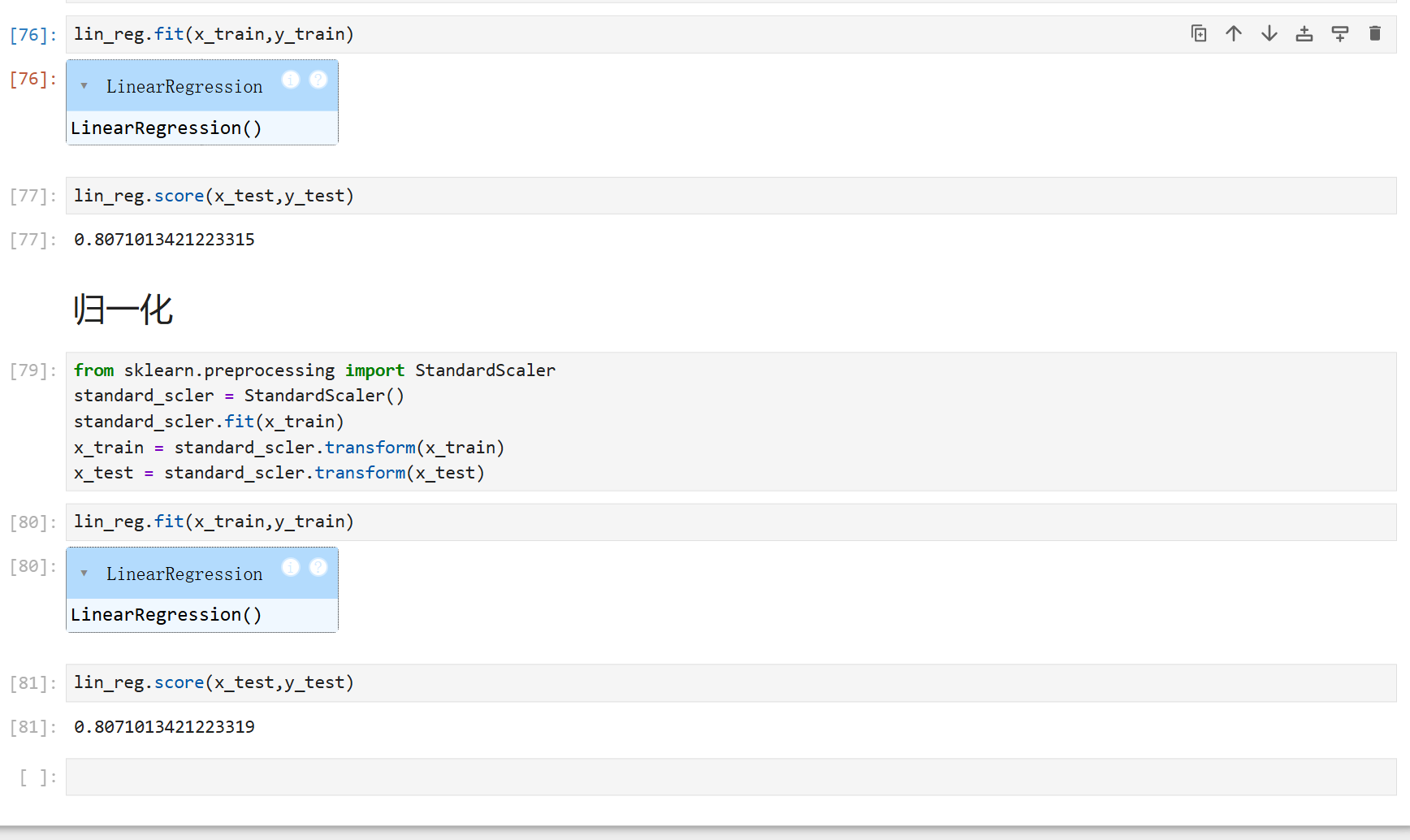
无需进行归一化操作（差别很小很小）

多项式回归        

# 构造非线性数据
import numpy as np
from sklearn import datasets
import matplotlib.pyplot as plt
from sklearn.model_selection import train_test_split

x = np.random.uniform(-4,2,size=(100))
y = 2*x*x + 4*x +3 +np.random.randn(100)

X = x.reshape(-1,1)
# 进行合并操作,水平合并
X_new = np.hstack([X,X**2])

lin_reg_new = LinearRegression()
lin_reg_new.fit(X_new,y)
y_predict_new = lin_reg_new.predict(X_new)
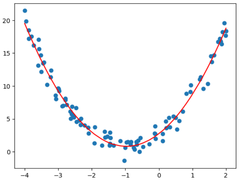
plt.scatter(x,y)
plt.plot(np.sort(x),y_predict_new[np.argsort(x)],c='r')
plt.show()

sklearn实现

from sklearn.preprocessing import PolynomialFeatures
# degree：多项式次数
polynormal_features = PolynomialFeatures(degree=2)
X_poly = polynormal_features.fit_transform(X)
lin_reg_poly = LinearRegression()
lin_reg_poly.fit(X_poly,y)
y_predict_poly = lin_reg_poly.predict(X_poly)

plt.scatter(x,y)
plt.plot(np.sort(x),y_predict_poly[np.argsort(x)],c='r')
plt.show()

线性回归的模型评价

• 均方误差（MSE--真值与预测值的差）:

• 均方根误差（RMSE）：

• 平均绝对误差（MAE）：

• RMSE和MAE的问题：
  • 无上限
  • 与数据取值相关
  • 只比较前后效果变化
• 判定系数（）

        即（TSS:方差np.var()）：

代码实现

# MSE
y_real = y_test
mse = np.sum((y_real-y_predict)**2)/(len(y_test))
# 使用sklearn计算MSE
from sklearn.metrics import mean_squared_error
mean_squared_error(y_real,y_predict)

# RMSE
rmse = np.sqrt(mse)

# MAE
mae = np.sum(np.abs(y_real-y_predict))/(len(y_real))
# 使用sklearn计算MAE
from sklearn.metrics import mean_absolute_error
mean_absolute_error(y_real,y_predict)

# R2
r2 = 1-np.sum((y_real-y_predict)**2)/np.sum((y_real-np.mean(y_real))**2)

1-mse/np.var(y_real)
# 要注意传入参数的顺序，第一个是真值，第二个是预测值
from sklearn.metrics import r2_score
r2_score(y_real,y_predict)
# score计算的便是R2
lin_reg.score(x_test,y_test)