机器学习就相当于数据的民主投票，选出一个能够代表这些数据的模型。

损失函数(Loss function)

平方损失函数：

绝对损失函数：

对数损失函数（二分类）：

交叉熵损失函数（多分类）：

• m:样本数，n：类别数，p：类别对应的概率，q：softmax函数

什么是熵

        熵（Entropy）用来度量数据的不确定性或混乱程度

• 信息熵：

• 相对熵（KL散度）：
  • 两个概率分布中的相似性

• 交叉熵：

• 经验风险（cost function）最小化准则:

• 添加正则化项：

梯度下降(优化算法)

• 梯度就是函数曲面的陡度
• 偏导数就是具体方向的陡度
• 梯度是所有方向偏导数向量和

学习率（步长）：

学习率太小，收敛慢，太大，不收敛

局部最优和全局最优：

• 极值点常常不唯一
• 随机初始化
• 初始点是超参数

常见梯度下降策略：

• 批量（BGD）：
  • 每次使用全部样本
  • 精确，但处理速度慢
• 随机梯度（SGD）：
  • 每次使用单个样本
  • 处理速度快，但不精确
• 小批量（MBGD）：
  • 每次使用小批量样本
  • 加快了速度，精确

决策边界

模型把不同类别样本分开的那条线 / 面 / 超平面。

逻辑回归的决策边界定义：

准备数据

import numpy as np
from sklearn import datasets
import matplotlib.pyplot as plt
from sklearn.model_selection import train_test_split
from sklearn.datasets import make_classification

x,y = make_classification(
    n_samples = 200,
    n_features = 2,
    n_redundant = 0,
    n_classes = 2,
    n_clusters_per_class=1,
    random_state = 1024
)
x_train,x_test,y_train,y_test=train_test_split(x,y,train_size=0.7,random_state=233,stratify=y)
from sklearn.linear_model import LogisticRegression
cls = LogisticRegression()
cls.fit(x_train,y_train)

仅绘制决策边界上的点

• cls.coef_[0] = [w1, w2]

• cls.intercept_ = w0

x1 = np.linspace(-4,4,1000)
x2 = (-cls.intercept_-cls.coef_[0][0]*x1)/cls.coef_[0][1]

# w1和w2
cls.coef_
# w0
cls.intercept_
plt.scatter(x_train[:,0],x_train[:,1],c=y_train)
plt.scatter(x1,x2)
plt.show()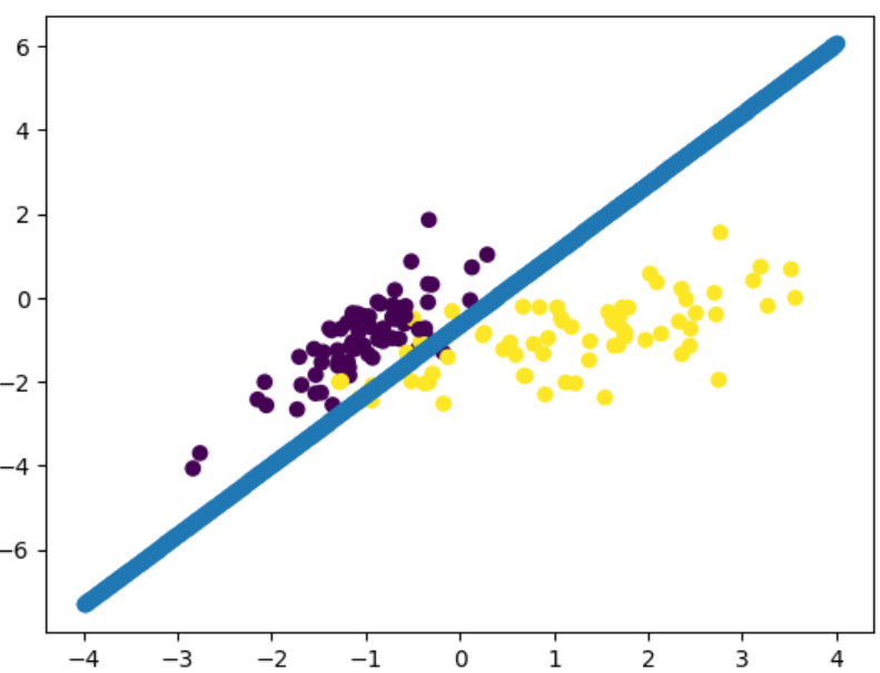

决策边界绘制函数：

def decision_boundary_plot(X,y,clf):
    axis_x1_min, axis_x1_max = X[:, 0].min() - 1, X[:, 0].max() + 1
    axis_x2_min, axis_x2_max = X[:, 1].min() - 1, X[:, 1].max() + 1
    x1, x2 = np.meshgrid(
        np.arange(axis_x1_min, axis_x1_max, 0.01),
        np.arange(axis_x2_min, axis_x2_max, 0.01),
    )
    z = clf.predict(np.c_[x1.ravel(), x2.ravel()])
    z = z.reshape(x1.shape)

    from matplotlib.colors import ListedColormap
    custom_cmap = ListedColormap(['#F5B9EF','#FFFFFF','#F9F9CB'])

    plt.contourf(x1,x2,z,cmap=custom_cmap)
    plt.scatter(X[:,0],X[:,1],c=y)

decision_boundary_plot(x,y,cls)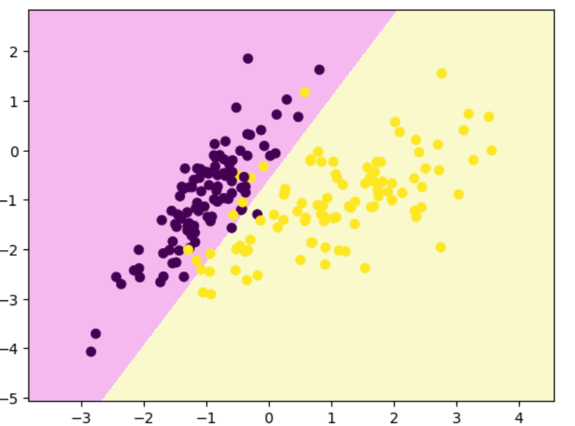

三分类决策边界(iris数据集)

iris = datasets.load_iris()
x = iris.data[:,:2]
y = iris.target
x_train,x_test,y_train,y_test=train_test_split(x,y,random_state=666)
cls.fit(x_train,y_train)
decision_boundary_plot(x,y,cls)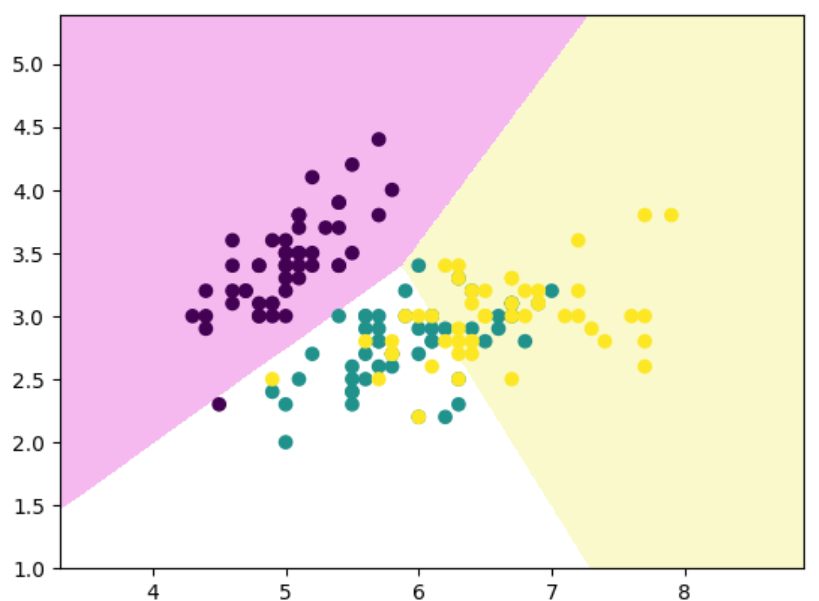

多项式逻辑回归决策边界

np.random.seed(0)
X = np.random.normal(0,1,size=(200,2))
y = np.array((X[:,0]**2)+(X[:,1]**2)<2,dtype='int')
x_train,x_test,y_train,y_test=train_test_split(X,y,train_size=0.7,random_state=233,stratify=y)

# 串联所有操作：Poly，归一化，逻辑回归...
from sklearn.pipeline import Pipeline
from sklearn.preprocessing import PolynomialFeatures
from sklearn.preprocessing import StandardScaler
clf_pipe = Pipeline([
    ('poly',PolynomialFeatures(degree=2)),
    ('std_scaler',StandardScaler()),
    ('log_reg',LogisticRegression())
])
clf_pipe.fit(x_train,y_train)
decision_boundary_plot(x_train,y_train,clf_pipe)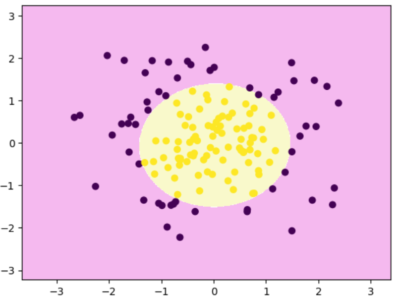

过拟合和欠拟合

过拟合：模型太复杂，把训练数据的“噪声”都当成规律记住了

欠拟合：模型太简单，连训练数据都学不好

欠拟合：学不会；过拟合：学太死。

数据准备：

import numpy as np
import matplotlib.pyplot as plt

np.random.seed(233)
x = np.random.uniform(-4,2,size=(100))
y = x**2 + 4*x +3 +2*np.random.randn(100)

X = x.reshape(-1,1)

欠拟合：

from sklearn.linear_model import LinearRegression
lin_reg = LinearRegression()

lin_reg.fit(X,y)
y_predict = lin_reg.predict(X)
plt.scatter(x,y)
plt.scatter(x,y_predict,c='r')
plt.show()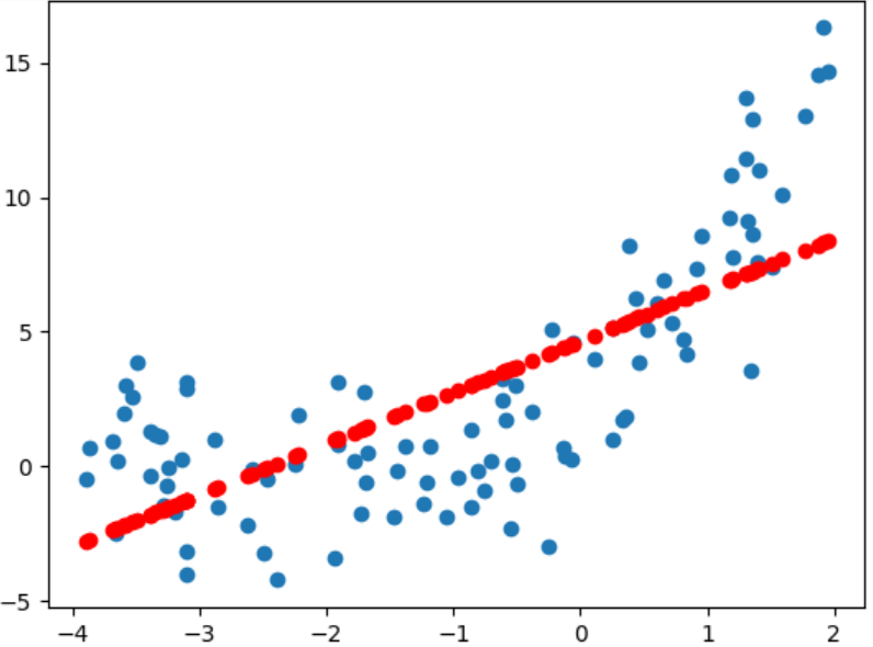

过拟合：

from sklearn.preprocessing import PolynomialFeatures
poly = PolynomialFeatures(degree=2)
poly.fit(X,y)
X_poly = poly.transform(X)
linear_reg = LinearRegression()
linear_reg.fit(X_poly,y)
y_predict_poly = linear_reg.predict(X_poly)
plt.scatter(x,y)
plt.plot(np.sort(x),y_predict_poly[np.argsort(x)],c='r')
plt.show()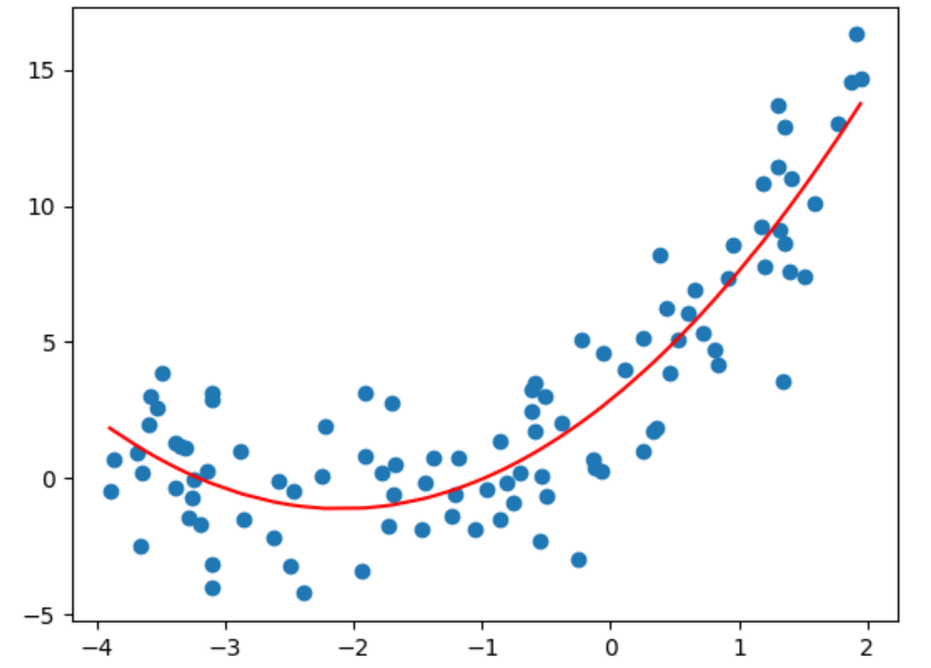

多项式次数不同”时，模型从欠拟合 → 合适 → 过拟合的全过程

degrees = [2,5,10,15,20,24]
plt.rcParams["figure.figsize"]=(12,8)

for i,degree in enumerate(degrees):
    poly = PolynomialFeatures(degree=degree)

    X_poly = poly.fit_transform(X)

    linear_reg = LinearRegression()
    linear_reg.fit(X_poly,y)
    
    X_new = np.linspace(-5,3,200).reshape(-1,1)
    X_new_poly = poly.fit_transform(X_new)
    y_predict = linear_reg.predict(X_new_poly)

    plt.subplot(2,3,i+1)
    plt.title("Degree:{0}".format(degree))
    plt.scatter(x,y)
    plt.ylim(-5,25)
    plt.plot(X_new,y_predict,c='r')
    

    print("Degree:",degree,"Score:",linear_reg.score(X_poly,y))

plt.show()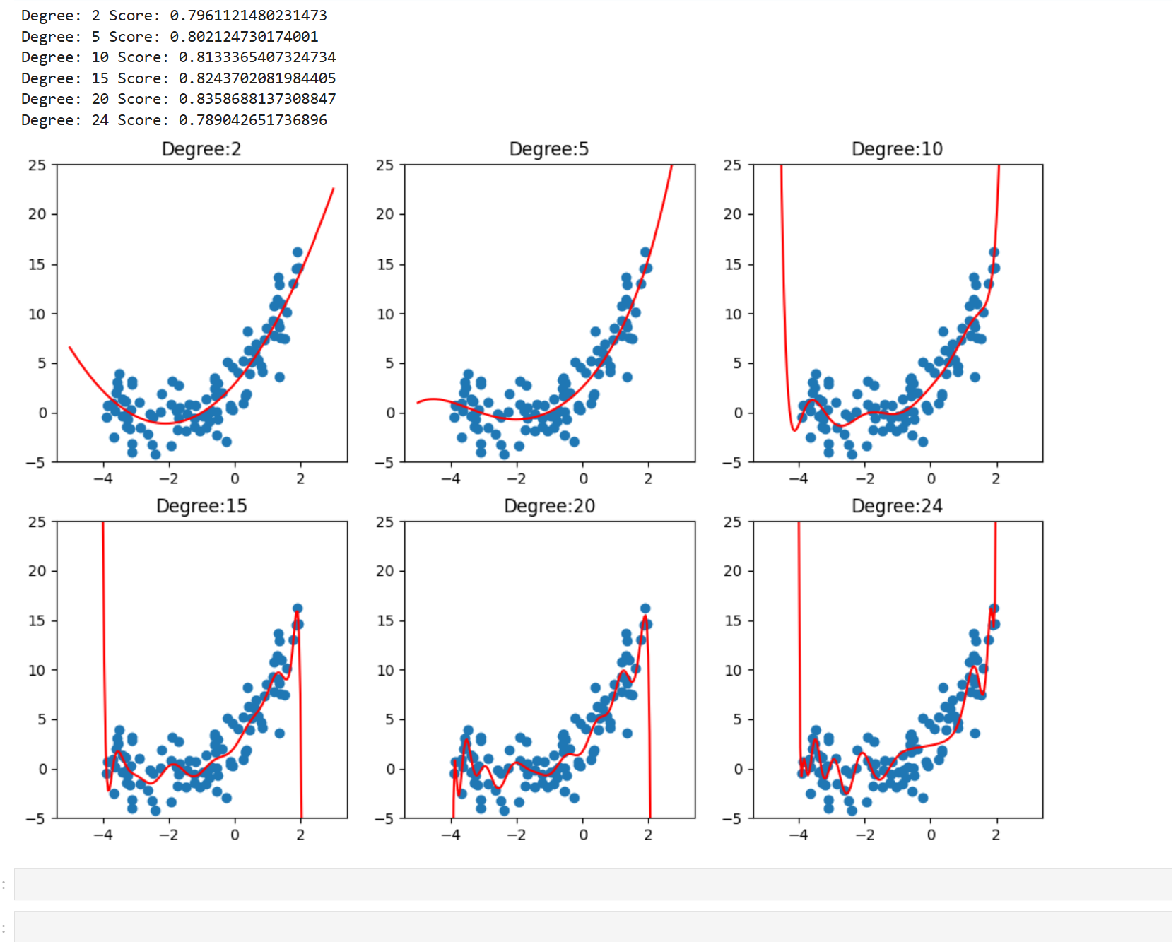

次数	现象	结论
2	曲线太平	欠拟合
5	较平滑	较合理
10	开始抖	风险上升
15+	剧烈震荡	明显过拟合

学习曲线

• 横轴是训练样本数量
• 纵轴是MSE均方误差
• 分别绘制训练和测试集误差（下面训练集，上面测试集）

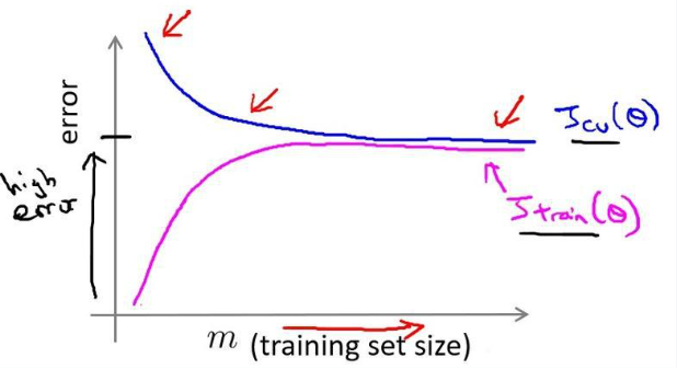
MSE(数据同上)

from sklearn.model_selection import train_test_split
x_train,x_test,y_train,y_test=train_test_split(x,y,train_size=0.7,random_state=233)
from sklearn.metrics import mean_squared_error

plt.rcParams["figure.figsize"]=(12,8)
degrees = [1,2,5,20]
for i,degree in enumerate(degrees):
    poly = PolynomialFeatures(degree=degree)

    x_poly_train = poly.fit_transform(x_train.reshape(-1,1))
    x_poly_test = poly.fit_transform(x_test.reshape(-1,1))
    
    train_error,test_error = [],[]
    for k in range(len(x_train)):
        linear_reg = LinearRegression()
        linear_reg.fit(x_poly_train[:k+1],y_train[:k+1])

        y_train_pred = linear_reg.predict(x_poly_train[:k+1])
        train_error.append(mean_squared_error(y_train[:k+1],y_train_pred))

        y_test_pred = linear_reg.predict(x_poly_test)
        test_error.append(mean_squared_error(y_test,y_test_pred))
    

    plt.subplot(2,2,i+1)
    plt.title("Degree:{0}".format(degree))
    plt.ylim(-5,50)
    plt.plot([k+1 for k in range(len(x_train))],train_error,c='r',label ='train')
    plt.plot([k+1 for k in range(len(x_train))],test_error,c='blue',label='test')

    plt.legend()

plt.show()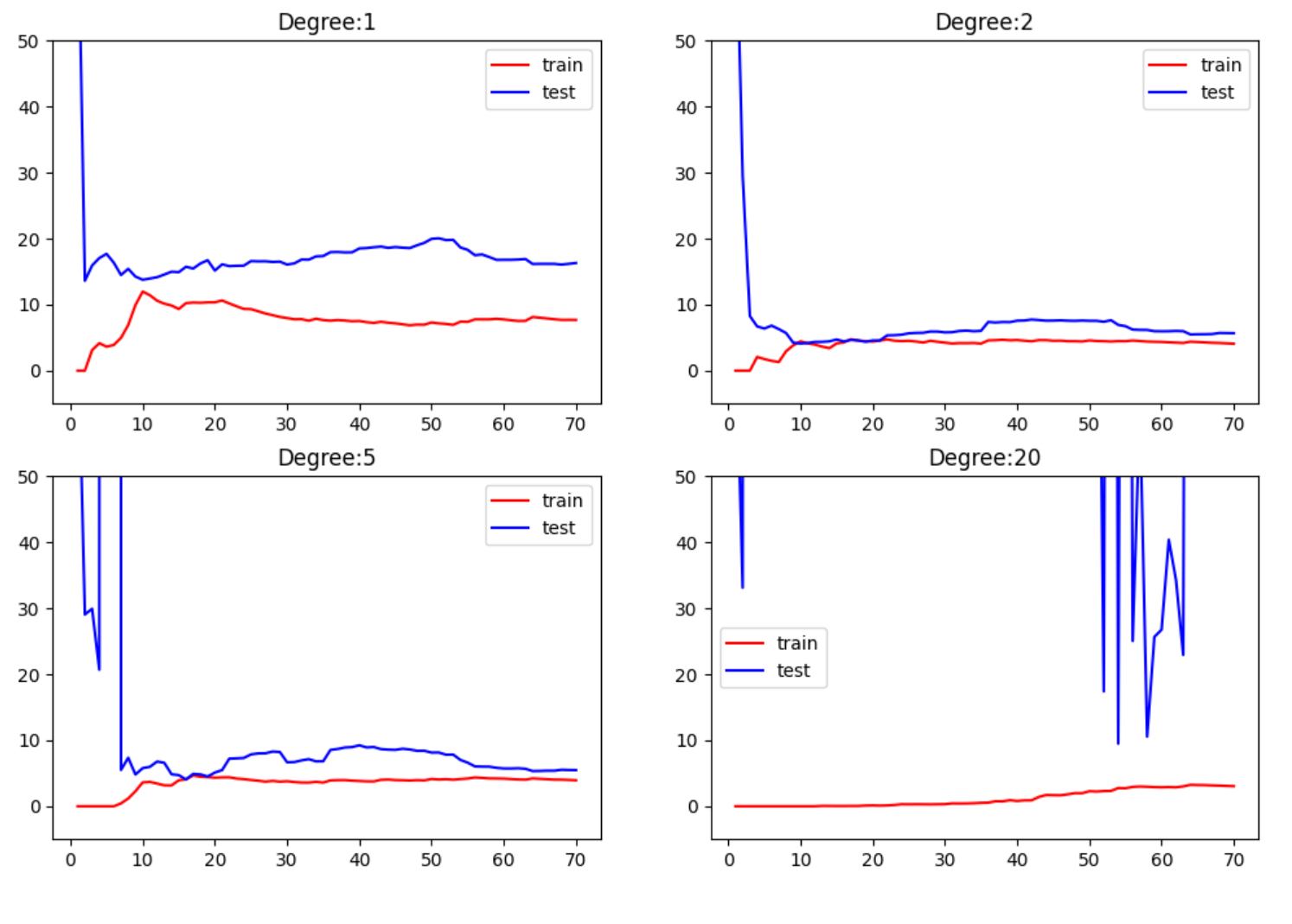

现象	说明
train 高，test 高	欠拟合
train 低，test 低	拟合合适
train 极低，test 高	过拟合
样本多 → test 下降	数据能缓解过拟合

from sklearn.metrics import mean_squared_error

plt.rcParams["figure.figsize"]=(12,8)
degrees = [1,2,5,20]
for i,degree in enumerate(degrees):
    poly = PolynomialFeatures(degree=degree)

    x_poly_train = poly.fit_transform(x_train.reshape(-1,1))
    x_poly_test = poly.fit_transform(x_test.reshape(-1,1))
    
    train_error,test_error = [],[]
    for k in range(1,len(x_train)):
        linear_reg = LinearRegression()
        linear_reg.fit(x_poly_train[:k+1],y_train[:k+1])

        train_error.append(linear_reg.score(x_poly_train[:k+1],y_train[:k+1]))

        test_error.append(linear_reg.score(x_poly_test,y_test))
    

    plt.subplot(2,2,i+1)
    plt.title("Degree:{0}".format(degree))
    plt.ylim(-1,1)
    plt.plot([k+1 for k in range(1,len(x_train))],train_error,c='r',label ='train')
    plt.plot([k+1 for k in range(1,len(x_train))],test_error,c='blue',label='test')

    plt.legend()

plt.show()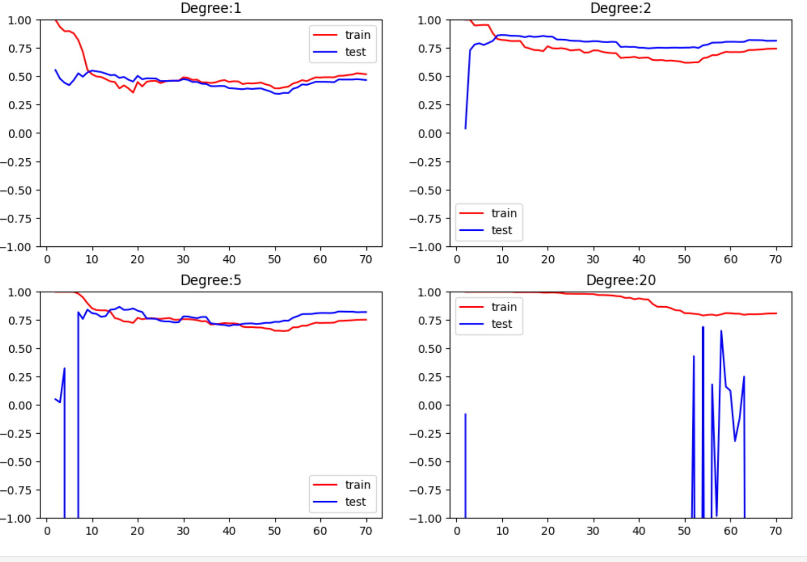

Degree	训练集 ()	测试集 ())	现象特征	结论
1	中等（≈0.4~0.5）	中等（≈0.4~0.5）	两条线接近、整体偏低	欠拟合
2	较高（≈0.75）	较高（≈0.8）	收敛稳定、间距小	最佳拟合
5	很高（≈0.85+）	略低（≈0.75~0.8）	间距扩大、初期不稳	轻度过拟合
20	接近 1	大幅震荡，甚至 < 0	极不稳定	严重过拟合

交叉验证

        模型恰巧在选择的测试集上效果好，但实际情况其实已经发生了过拟合，这样的情况下，准确率和学习曲线的表现看似良好，但当使用真实数据的时候效果就可能很差。

        解决方法：把训练集再抽出一组作为验证集，使用训练集(练习题)训练模型，验证集(模拟测验检验学习方法是否正确)搜索最优超参数，然后最后使用测试集(最终考试)评价最终效果

K-fold交叉验证

验证集准确率均值（测试集：黄色，验证集：绿色，训练集：蓝色）

数据准备：

import numpy as np
from sklearn import datasets
import matplotlib.pyplot as plt
from sklearn.model_selection import train_test_split

iris =datasets.load_iris()
x = iris.data
y = iris.target
x_train,x_test,y_train,y_test=train_test_split(x,y,train_size=0.7,random_state=233,stratify=y)

交叉验证(超参数搜索)

from sklearn.model_selection import cross_val_score
# 把传入的训练样本分成5份，对 KNN 模型做 5 折交叉验证，并返回每一折的得分
neigh = KNeighborsClassifier()
cv_score = cross_val_score(neigh,x_train,y_train,cv=5)
best_score = -1
best_n = -1
best_weight = ''
best_p = -1
best_cv_scores = None
for n in range(1,20):
    for weight in ['uniform','distance']:
        for p in range(1,7):
            neigh = KNeighborsClassifier(
                n_neighbors=n,
                weights=weight,
                p=p
            )
            neigh.fit(x_train,y_train)
            cv_score = cross_val_score(neigh,x_train,y_train,cv=5)
            score = np.mean(cv_score)
            if score > best_score:
                best_score = score
                best_n = n
                best_weight = weight
                best_p = p
                best_cv_scores = cv_score
print("best_n:",best_n)
print("best_weight:",best_weight)
print("best_p:",best_p)
print("best_score:",best_score)
print("best_cv_scores:",best_cv_scores)