1、numpy

1.1、np.where

x = np.array([[1, 2], [3, 4]])
print(np.where(x > 2, True, False))

# 打印结果
[[False False]
 [ True  True]]

1.2、@运算

# 2D X 2D
A = np.random.rand(3, 4)
B = np.random.rand(4, 5)
C = A @ B
print("2D X 2D:", A.shape, "X", B.shape, "=", C.shape)

# 3D X 3D
A = np.random.rand(10, 3, 4)
B = np.random.rand(10, 4, 5)
C = A @ B
print("3D X 3D:", A.shape, "X", B.shape, "=", C.shape)

# 3D X 4D
A = np.random.rand(2, 3, 4)      # shape (2, 3, 4) → 3D
B = np.random.rand(5, 2, 4, 6)   # shape (5, 2, 4, 6) → 4D
# 要求：A.shape[-1] == B.shape[-2]
C = A @ B
print("3D X 4D:", A.shape, "X", B.shape, "=", C.shape)

# 3D X 4D
A = np.random.rand(1, 3, 4)      # shape (2, 3, 4) → 3D
B = np.random.rand(5, 2, 4, 6)   # shape (5, 2, 4, 6) → 4D
# 要求：A.shape[-1] == B.shape[-2]
C = A @ B
print("3D X 4D:", A.shape, "X", B.shape, "=", C.shape)

# 3D X 4D
A = np.random.rand(2, 3, 4)      # shape (2, 3, 4) → 3D
B = np.random.rand(5, 1, 4, 6)   # shape (5, 2, 4, 6) → 4D
# 要求：A.shape[-1] == B.shape[-2]
C = A @ B
print("3D X 4D:", A.shape, "X", B.shape, "=", C.shape)

# 4D X 3D
A = np.random.rand(5, 3, 4, 6)   # shape (5, 2, 4, 6) → 4D
B = np.random.rand(3, 6, 4)      # shape (2, 3, 4) → 3D
# 要求：A.shape[-1] == B.shape[-2]
C = A @ B
print("4D X 3D:", A.shape, "X", B.shape, "=", C.shape)

# 4D X 3D
A = np.random.rand(5, 1, 4, 6)   # shape (5, 2, 4, 6) → 4D
B = np.random.rand(3, 6, 4)      # shape (2, 3, 4) → 3D
# 要求：A.shape[-1] == B.shape[-2]
C = A @ B
print("4D X 3D:", A.shape, "X", B.shape, "=", C.shape)

# 4D X 3D
A = np.random.rand(5, 3, 4, 6)   # shape (5, 2, 4, 6) → 4D
B = np.random.rand(1, 6, 4)      # shape (2, 3, 4) → 3D
# 要求：A.shape[-1] == B.shape[-2]
C = A @ B
print("4D X 3D:", A.shape, "X", B.shape, "=", C.shape)

# 3D X 4D
A = np.random.rand(3, 3, 4)      # shape (2, 3, 4) → 3D
B = np.random.rand(5, 2, 4, 6)   # shape (5, 2, 4, 6) → 4D
# 要求：A.shape[-1] == B.shape[-2]
try: 
    C = A @ B
    print("3D X 4D:", A.shape, "X", B.shape, "=", C.shape)
except ValueError as e:
    print("❌ 3D X 4D 失败！")
    print("   提示：A.shape[-1] == B.shape[-2]")
    print("        确保批处理维度可以广播。")
    print("   广播规则1：广播从右向左对齐, 不包括最后两维")
    print("   广播规则2：维度要么相等，要么其中一个是 1，否则报错")
    print("   详细错误：", e)
    
# 4D X 3D
A = np.random.rand(5, 3, 4, 6)   # shape (5, 2, 4, 6) → 4D
B = np.random.rand(2, 6, 4)      # shape (2, 3, 4) → 3D
# 要求：A.shape[-1] == B.shape[-2]
try: 
    C = A @ B
    print("3D X 4D:", A.shape, "X", B.shape, "=", C.shape)
except ValueError as e:
    print("❌ 4D X 3D 失败！")
    print("   提示：A.shape[-1] == B.shape[-2]")
    print("        确保批处理维度可以广播。")
    print("   广播规则1：广播从右向左对齐, 不包括最后两维")
    print("   广播规则2：维度要么相等，要么其中一个是 1，否则报错")
    print("   详细错误：", e)

# 打印结果
2D X 2D: (3, 4) X (4, 5) = (3, 5)
3D X 3D: (10, 3, 4) X (10, 4, 5) = (10, 3, 5)
3D X 4D: (2, 3, 4) X (5, 2, 4, 6) = (5, 2, 3, 6)
3D X 4D: (1, 3, 4) X (5, 2, 4, 6) = (5, 2, 3, 6)
3D X 4D: (2, 3, 4) X (5, 1, 4, 6) = (5, 2, 3, 6)
4D X 3D: (5, 3, 4, 6) X (3, 6, 4) = (5, 3, 4, 4)
4D X 3D: (5, 1, 4, 6) X (3, 6, 4) = (5, 3, 4, 4)
4D X 3D: (5, 3, 4, 6) X (1, 6, 4) = (5, 3, 4, 4)
❌ 3D X 4D 失败！
   提示：A.shape[-1] == B.shape[-2]
        确保批处理维度可以广播。
   广播规则1：广播从右向左对齐, 不包括最后两维
   广播规则2：维度要么相等，要么其中一个是 1，否则报错
   详细错误： operands could not be broadcast together with remapped shapes [original->remapped]: (3,3,4)->(3,newaxis,newaxis) (5,2,4,6)->(5,2,newaxis,newaxis)  and requested shape (3,6)
❌ 4D X 3D 失败！
   提示：A.shape[-1] == B.shape[-2]
        确保批处理维度可以广播。
   广播规则1：广播从右向左对齐, 不包括最后两维
   广播规则2：维度要么相等，要么其中一个是 1，否则报错
   详细错误： operands could not be broadcast together with remapped shapes [original->remapped]: (5,3,4,6)->(5,3,newaxis,newaxis) (2,6,4)->(2,newaxis,newaxis)  and requested shape (4,4)

1.3、np.arange

np.arange(0,10)
np.arange(0,10,2)

# 打印结果
array([0, 1, 2, 3, 4, 5, 6, 7, 8, 9])
array([0, 2, 4, 6, 8])

1.4、随机数生

1.4.1、随机数生成

# 正太分布
np.random.normal(loc=[6, 2.5], scale=[0.5, 0.5], size=(50, 2)).shape
# 标准正太分布
np.random.rand(50,2).shape

# 打印结果
(50, 2)
(50, 2)

1.4.2、随机种子

rgen = np.random.RandomState(666)
rgen.normal(loc=[5, 1], scale=[0.5, 0.5], size=(50, 2)).shape

# 打印结果
(50, 2)

或者

np.random.seed(0)
np.random.normal(loc=[5, 1], scale=[0.5, 0.5], size=(50, 2)).shape

# 打印结果
(50, 2)

1.5、矩阵拼接

1.5.1、np.vstack

拼接第0维，其余维度要完全一致

x = np.random.rand(9,2,3,4)
y = np.random.rand(2,2,3,4)
np.vstack((y,x)).shape

# 打印结果
(11, 2, 3, 4)

1.5.2、np.hstack

拼接第1维，其余维度要完全一致

x = np.random.rand(66,9,2,3,4)
y = np.random.rand(66,3,2,3,4)
np.hstack((y,x)).shape

# 打印结果
(66, 12, 2, 3, 4)

1.5.3、np.concatenate

拼接指定的axis维，除了axis维，其余维度要完全一致

x = np.random.rand(9,2,1,4)
y = np.random.rand(9,2,3,4)
np.concatenate((x,y), axis=2).shape

# 打印结果
(9, 2, 4, 4)

1.5.4、np.stack

把多个形状相同的数组，沿着一个新轴axis堆叠起来，形成更高维的数组。

axis	输出形状	含义
0	(N, 1, 2, 3, 4)	在最前面加一维
1	(1, N, 2, 3, 4)
2	(1, 2, N, 3, 4)
3	(1, 2, 3, N, 4)
4	(1, 2, 3, 4, N)	在最后面加一维

a = np.random.rand(1,2,3,4)
b = np.random.rand(1,2,3,4)
print(np.stack((a, b), axis=0).shape)
print(np.stack((a, b), axis=1).shape)
print(np.stack((a, b), axis=2).shape)
print(np.stack((a, b), axis=3).shape)
print(np.stack((a, b), axis=4).shape)

# 打印结果
(2, 1, 2, 3, 4)
(1, 2, 2, 3, 4)
(1, 2, 2, 3, 4)
(1, 2, 3, 2, 4)
(1, 2, 3, 4, 2)

1.6、求最值

1.6.1、np.argmax（最大值）

x = np.random.rand(32, 100)
x.argmax(axis=0).shape
x.argmax(axis=1).shape

# 打印结果
(100,)
(32,)

1.6.2、np.argmin（最小值）

x = np.random.rand(32, 100)
x.argmin(axis=0).shape
x.argmin(axis=1).shape

# 打印结果
(100,)
(32,)

1.7、np.reshape

x = np.random.rand(32,3,224,224)
x.reshape(32*3,224,224).shape
x.reshape(32*3,-1).shape

# 打印结果
(96, 224, 224)
(96, 50176)

1.8、排序

1.8.1、np.sort（排序结果）

升序

x = np.array([[7,2,3],[6,5,4]])
x.shape
np.sort(x, axis=0)
np.sort(x, axis=1)

# 打印结果
(2, 3)
array([[6, 2, 3],
       [7, 5, 4]])

array([[2, 3, 7],
       [4, 5, 6]])

降序

x = np.array([[7,2,3],[6,5,4]])
x.shape
np.sort(x, axis=0)[::-1, :]
np.sort(x, axis=1)[:, ::-1]

# 打印结果
(2, 3)
array([[7, 5, 4],
       [6, 2, 3]])

array([[7, 3, 2],
       [6, 5, 4]])

1.8.2、np.argsort（排序索引）

升序

x = np.array([[7,2,3],[6,5,4]])
x.shape
np.argsort(x, axis=0)
np.argsort(x, axis=1)

# 打印结果
(2, 3)
array([[1, 0, 0],
       [0, 1, 1]], dtype=int64)
       
array([[1, 2, 0],
       [2, 1, 0]], dtype=int64)

降序

x = np.array([[7,2,3],[6,5,4]])
x.shape
np.argsort(x, axis=0)[::-1,:]
np.argsort(x, axis=1)[:,::-1]

# 打印结果
(2, 3)
array([[1, 0, 0],
       [0, 1, 1]], dtype=int64)
       
array([[0, 2, 1],
       [0, 1, 2]], dtype=int64)

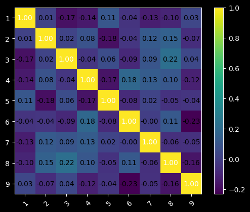
1.9、np.corrcoef（皮尔逊积矩相关系数）

name = ['1','2','3','4','5','6','7','8','9']
cwb = np.random.rand(9, 100)
cmcwb = np.corrcoef(cwb)
hm = heatmap(cmcwb, row_names=name, column_names=name)
cmcwb.shape

# 打印结果
(9, 9)

1.10、np.flatten

import numpy as np
arr = np.array([[1, 2, 3], [4, 5, 6]])
print("原始数组:\n", arr)
print("按行优先展平后的数组:", arr.flatten())
print("按列优先展平后的数组:", arr.flatten(order='F'))

原始数组:
 [[1 2 3]
 [4 5 6]]
按行优先展平后的数组: [1 2 3 4 5 6]
按列优先展平后的数组: [1 4 2 5 3 6]

2、pytorch

2.1、torch.where

x = torch.rand(3,4)
print(x)
print(torch.where(x > 0.1, True, False))

tensor([[0.1676, 0.1753, 0.8944, 0.0824],
        [0.7810, 0.7906, 0.8193, 0.7872],
        [0.7148, 0.1584, 0.9870, 0.9250]])
tensor([[ True,  True,  True, False],
        [ True,  True,  True,  True],
        [ True,  True,  True,  True]])

2.2、torch.matmul（矩阵乘法）

# 2D X 2D
A = torch.rand(3, 4)
B = torch.rand(4, 5)
C = torch.matmul(A,B)
print("2D X 2D:", A.shape, "X", B.shape, "=", C.shape)

# 3D X 3D
A = torch.rand(10, 3, 4)
B = torch.rand(10, 4, 5)
C = torch.matmul(A,B)
print("3D X 3D:", A.shape, "X", B.shape, "=", C.shape)

# 3D X 4D
A = torch.rand(2, 3, 4)      # shape (2, 3, 4) → 3D
B = torch.rand(5, 2, 4, 6)   # shape (5, 2, 4, 6) → 4D
# 要求：A.shape[-1] == B.shape[-2]
C = torch.matmul(A,B)
print("3D X 4D:", A.shape, "X", B.shape, "=", C.shape)

# 3D X 4D
A = torch.rand(1, 3, 4)      # shape (2, 3, 4) → 3D
B = torch.rand(5, 2, 4, 6)   # shape (5, 2, 4, 6) → 4D
# 要求：A.shape[-1] == B.shape[-2]
C = torch.matmul(A,B)
print("3D X 4D:", A.shape, "X", B.shape, "=", C.shape)

# 3D X 4D
A = torch.rand(2, 3, 4)      # shape (2, 3, 4) → 3D
B = torch.rand(5, 1, 4, 6)   # shape (5, 2, 4, 6) → 4D
# 要求：A.shape[-1] == B.shape[-2]
C = torch.matmul(A,B)
print("3D X 4D:", A.shape, "X", B.shape, "=", C.shape)

# 4D X 3D
A = torch.rand(5, 3, 4, 6)   # shape (5, 2, 4, 6) → 4D
B = torch.rand(3, 6, 4)      # shape (2, 3, 4) → 3D
# 要求：A.shape[-1] == B.shape[-2]
C = torch.matmul(A,B)
print("4D X 3D:", A.shape, "X", B.shape, "=", C.shape)

# 4D X 3D
A = torch.rand(5, 1, 4, 6)   # shape (5, 2, 4, 6) → 4D
B = torch.rand(3, 6, 4)      # shape (2, 3, 4) → 3D
# 要求：A.shape[-1] == B.shape[-2]
C = torch.matmul(A,B)
print("4D X 3D:", A.shape, "X", B.shape, "=", C.shape)

# 4D X 3D
A = torch.rand(5, 3, 4, 6)   # shape (5, 2, 4, 6) → 4D
B = torch.rand(1, 6, 4)      # shape (2, 3, 4) → 3D
# 要求：A.shape[-1] == B.shape[-2]
C = torch.matmul(A,B)
print("4D X 3D:", A.shape, "X", B.shape, "=", C.shape)

# 3D X 4D
A = torch.rand(3, 3, 4)      # shape (2, 3, 4) → 3D
B = torch.rand(5, 2, 4, 6)   # shape (5, 2, 4, 6) → 4D
# 要求：A.shape[-1] == B.shape[-2]
try: 
    C = torch.matmul(A,B)
    print("3D X 4D:", A.shape, "X", B.shape, "=", C.shape)
except RuntimeError as e:
    print("❌ 3D X 4D 失败！")
    print("   提示：A.shape[-1] == B.shape[-2]")
    print("        确保批处理维度可以广播。")
    print("   广播规则1：广播从右向左对齐, 不包括最后两维")
    print("   广播规则2：维度要么相等，要么其中一个是 1，否则报错")
    print("   详细错误：", e)
    
# 4D X 3D
A = torch.rand(5, 3, 4, 6)   # shape (5, 2, 4, 6) → 4D
B = torch.rand(2, 6, 4)      # shape (2, 3, 4) → 3D
# 要求：A.shape[-1] == B.shape[-2]
try: 
    C = torch.matmul(A,B)
    print("3D X 4D:", A.shape, "X", B.shape, "=", C.shape)
except RuntimeError as e:
    print("❌ 4D X 3D 失败！")
    print("   提示：A.shape[-1] == B.shape[-2]")
    print("        确保批处理维度可以广播。")
    print("   广播规则1：广播从右向左对齐, 不包括最后两维")
    print("   广播规则2：维度要么相等，要么其中一个是 1，否则报错")
    print("   详细错误：", e)

2D X 2D: torch.Size([3, 4]) X torch.Size([4, 5]) = torch.Size([3, 5])
3D X 3D: torch.Size([10, 3, 4]) X torch.Size([10, 4, 5]) = torch.Size([10, 3, 5])
3D X 4D: torch.Size([2, 3, 4]) X torch.Size([5, 2, 4, 6]) = torch.Size([5, 2, 3, 6])
3D X 4D: torch.Size([1, 3, 4]) X torch.Size([5, 2, 4, 6]) = torch.Size([5, 2, 3, 6])
3D X 4D: torch.Size([2, 3, 4]) X torch.Size([5, 1, 4, 6]) = torch.Size([5, 2, 3, 6])
4D X 3D: torch.Size([5, 3, 4, 6]) X torch.Size([3, 6, 4]) = torch.Size([5, 3, 4, 4])
4D X 3D: torch.Size([5, 1, 4, 6]) X torch.Size([3, 6, 4]) = torch.Size([5, 3, 4, 4])
4D X 3D: torch.Size([5, 3, 4, 6]) X torch.Size([1, 6, 4]) = torch.Size([5, 3, 4, 4])
❌ 3D X 4D 失败！
   提示：A.shape[-1] == B.shape[-2]
        确保批处理维度可以广播。
   广播规则1：广播从右向左对齐, 不包括最后两维
   广播规则2：维度要么相等，要么其中一个是 1，否则报错
   详细错误： The size of tensor a (3) must match the size of tensor b (2) at non-singleton dimension 1
❌ 4D X 3D 失败！
   提示：A.shape[-1] == B.shape[-2]
        确保批处理维度可以广播。
   广播规则1：广播从右向左对齐, 不包括最后两维
   广播规则2：维度要么相等，要么其中一个是 1，否则报错
   详细错误： The size of tensor a (3) must match the size of tensor b (2) at non-singleton dimension 1

2.3、torch.multiply（矩阵点积）

# 2D X 2D
A = torch.rand(3, 4)
B = torch.rand(3, 4)
C = torch.multiply(A,B)
print("2D X 2D:", A.shape, "X", B.shape, "=", C.shape)

# 打印结果
2D X 2D: torch.Size([3, 4]) X torch.Size([3, 4]) = torch.Size([3, 4])

2.4、torch.arange

# 2D X 2D
print(torch.arange(0, 10, dtype=torch.float32))
print(torch.arange(0, 10, 2, dtype=torch.float32))

# 打印结果
tensor([0., 1., 2., 3., 4., 5., 6., 7., 8., 9.])
tensor([0., 2., 4., 6., 8.])

2.5、随机数生

2.5.1、随机数生成

# 正太分布
mean = torch.tensor([6.0, 2.5]).expand(50, 2)
std = torch.tensor([0.5, 0.5]).expand(50, 2)
torch.normal(mean=mean, std=std).shape
# 标准正太分布
torch.rand(50, 2).shape

# 打印结果
(50, 2)
(50, 2)

2.5.2、随机种子

generator = torch.Generator()
generator.manual_seed(666)
torch.rand([50, 2], generator=generator).shape

# 打印结果
(50, 2)

或者

torch.manual_seed(22)
torch.rand([50, 2]).shape

# 打印结果
(50, 2)

2.6、矩阵拼接

2.6.1、torch.cat

A = torch.rand(32,3,224,224)
B = torch.rand(32,3,224,224)
print(torch.cat([A, B], axis=0).shape)
print(torch.cat([A, B], axis=1).shape)
print(torch.cat([A, B], axis=2).shape)
print(torch.cat([A, B], axis=3).shape)

# 打印结果
torch.Size([64, 3, 224, 224])
torch.Size([32, 6, 224, 224])
torch.Size([32, 3, 448, 224])
torch.Size([32, 3, 224, 448])

2.6.2、torch.stack

把多个形状相同的数组，沿着一个新轴axis堆叠起来，形成更高维的数组。

axis	输出形状	含义
0	(N, 1, 2, 3, 4)	在最前面加一维
1	(1, N, 2, 3, 4)
2	(1, 2, N, 3, 4)
3	(1, 2, 3, N, 4)
4	(1, 2, 3, 4, N)	在最后面加一维

A = torch.rand(32,3,224,224)
B = torch.rand(32,3,224,224)
print(torch.stack([A, B], axis=0).shape)
print(torch.stack([A, B], axis=1).shape)
print(torch.stack([A, B], axis=2).shape)
print(torch.stack([A, B], axis=3).shape)
print(torch.stack([A, B], axis=4).shape)

# 打印结果
torch.Size([2, 32, 3, 224, 224])
torch.Size([32, 2, 3, 224, 224])
torch.Size([32, 3, 2, 224, 224])
torch.Size([32, 3, 224, 2, 224])
torch.Size([32, 3, 224, 224, 2])

2.7、求最值

2.7.1、torch.argmax / torch.argmin（最值）

A = torch.tensor([[3,1,2],[4,6,5]])
print(torch.argmax(A, dim=0), torch.argmax(A, dim=0).shape)
print(torch.argmax(A, dim=1), torch.argmax(A, dim=1).shape)

# 打印结果
tensor([1, 1, 1]) torch.Size([3])
tensor([0, 1]) torch.Size([2])

2.7.2、torch.max / torch.min（最值）

A = torch.tensor([[3,1,2],[4,6,5]])
print(A.max(dim=0).values)
print(A.max(dim=0).indices)

# 打印结果
tensor([4, 6, 5])
tensor([1, 1, 1])

2.8、torch.reshape

x = torch.rand(32,3,224,224)
print(x.reshape(32*3,224,224).shape)
print(x.reshape(32*3,-1).shape)

# 打印结果
torch.Size([96, 224, 224])
torch.Size([96, 50176])

2.9、排序

2.9.1、np.sort（排序结果）

升序

A = torch.tensor([[3,1,2], [4,6,5]])
print(torch.sort(A, dim=0).values)
print(torch.sort(A, dim=0).indices)
print('--------------------------')
print(torch.sort(A, dim=1).values)
print(torch.sort(A, dim=1).indices)

# 打印结果
(2, 3)
tensor([[3, 1, 2],
        [4, 6, 5]])
tensor([[0, 0, 0],
        [1, 1, 1]])
--------------------------
tensor([[1, 2, 3],
        [4, 5, 6]])
tensor([[1, 2, 0],
        [0, 2, 1]])

降序

A = torch.tensor([[3,1,2], [4,6,5]])
print(torch.sort(A, dim=0, descending=True).values)
print(torch.sort(A, dim=0, descending=True).indices)
print('--------------------------')
print(torch.sort(A, dim=1, descending=True).values)
print(torch.sort(A, dim=1, descending=True).indices)

# 打印结果
tensor([[4, 6, 5],
        [3, 1, 2]])
tensor([[1, 1, 1],
        [0, 0, 0]])
--------------------------
tensor([[3, 2, 1],
        [6, 5, 4]])
tensor([[0, 2, 1],
        [1, 2, 0]])

2.9.2、np.argsort（排序索引）

升序

A = torch.tensor([[3,1,2], [4,6,5]])
print(torch.argsort(A, dim=0))
print(torch.argsort(A, dim=1))

# 打印结果
tensor([[0, 0, 0],
        [1, 1, 1]])
        
tensor([[1, 2, 0],
        [0, 2, 1]])

降序

A = torch.tensor([[3,1,2], [4,6,5]])
print(torch.argsort(A, dim=0, descending=True))
print(torch.argsort(A, dim=1, descending=True))

# 打印结果
(2, 3)
tensor([[1, 1, 1],
        [0, 0, 0]])
        
tensor([[0, 2, 1],
        [1, 2, 0]])

2.10、（L1，L2，…）范数

A = torch.tensor([[-1,2,3],[4,-5,6]], dtype=torch.float32)
print('A = ', A)
print('A dim=1 L1范数：', torch.linalg.norm(A, ord=1, dim=1))
print('A dim=0 L2范数：', torch.linalg.norm(A, ord=2, dim=0))

# 打印结果
A =  tensor([[-1.,  2.,  3.],
        [ 4., -5.,  6.]])
A dim=1 L1范数： tensor([ 6., 15.])
A dim=0 L2范数： tensor([4.1231, 5.3852, 6.7082])

2.11、torch.flatten

A = torch.rand(32,3,224,224)
A.flatten(start_dim = 0, end_dim=1).shape

torch.Size([96, 224, 224])

2.12、torch.permute / torch.transpose（调换维度）

x = torch.rand(32, 3, 224, 224)
print(x.shape) # [32, 3, 224, 224]
print(x.permute(0, 2, 3, 1).shape) # 重排 [32, 3, 224, 224] -> [32, 224, 224, 3]
print(x.transpose(0, 3).shape) # 交换 [32, 3, 224, 224] -> [224, 3, 224, 32]

torch.Size([32, 3, 224, 224])
torch.Size([32, 224, 224, 3])
torch.Size([224, 3, 224, 32])

2.13、transforms、Dataset、DataLoader（数据加载器，编程模板）

from torch.utils.data import Dataset, DataLoader
import torchvision.transforms as transforms
import torch

x = torch.arange(0,5)
y = torch.cat((torch.ones(2), torch.zeros(3)), dim=0)

myTransform = transforms.Compose([
    transforms.ToTensor(),  # 转换为Tensor + 每个值除以255 -> 缩放到 [0, 1]，
    transforms.Normalize(
        mean=[0.485, 0.456, 0.406],
        std=[0.229, 0.224, 0.225])  # 标准化
])

class MyDatesets(Dataset):
    def __init__(self, x, y, transform=None):
        self.x = x
        self.y = y
        self.transform = transform

    def __getitem__(self, index):
        if self.transform is None:
            return x[index], y[index]
        else:
            return self.transform(x[index]), self.transform(y[index])

    def __len__(self):
        return len(y)

if __name__ == '__main__':
    torch.manual_seed(666)
    
    myDataLoader = DataLoader(
        dataset=MyDatesets(x,y),
        batch_size=2,
        shuffle=True,
        drop_last=True,
    )

    load_sample_count = 0
    for i, (xi, yi) in enumerate(myDataLoader):
        print('xi = ', xi, 'yi = ', yi)
        load_sample_count += len(yi)

    print('被丢弃的样本数量 = ', 5 - load_sample_count, '\n')

    load_sample_count = 0
    for i, (xi, yi) in enumerate(myDataLoader):
        print('xi = ', xi, 'yi = ', yi)
        load_sample_count += len(yi)

    print('被丢弃的样本数量 = ', 5 - load_sample_count)

# 打印输出
xi =  tensor([2, 0]) yi =  tensor([0., 1.])
xi =  tensor([4, 3]) yi =  tensor([0., 0.])
被丢弃的样本数量 =  1

xi =  tensor([0, 1]) yi =  tensor([1., 1.])
xi =  tensor([3, 4]) yi =  tensor([0., 0.])
被丢弃的样本数量 =  1

3、matplotlib

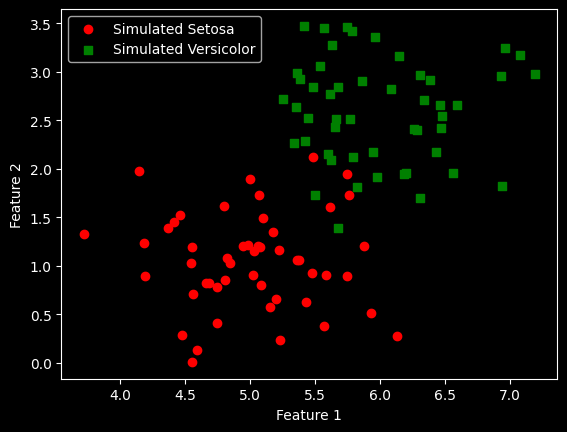
3.1、散点图

import numpy as np
import matplotlib.pyplot as plt

# 设置随机种子以便结果可复现
np.random.seed(0)

# 生成第一组数据（模拟'Iris-setosa'）
# (50,2)
data_setosa = np.random.normal(loc=[5, 1], scale=[0.5, 0.5], size=(50, 2))

# 生成第二组数据（模拟'Versicolor'）
# (50,2)
data_versicolor = np.random.normal(loc=[6, 2.5], scale=[0.5, 0.5], size=(50, 2))

# 合并数据
# (100,2)
x = np.vstack((data_setosa, data_versicolor))

# 创建标签
# (100,)
y = np.hstack((np.zeros(50), np.ones(50)))

# 绘制散点图
plt.scatter(x[:50, 0], x[:50, 1], color='red', marker='o', label='Simulated Setosa')
plt.scatter(x[50:100, 0], x[50:100, 1], color='green', marker='s', label='Simulated Versicolor')

# 添加轴标签和图例
plt.xlabel('Feature 1')
plt.ylabel('Feature 2')
plt.legend(loc='upper left')

# 显示图形
plt.show()

3.2、多张图

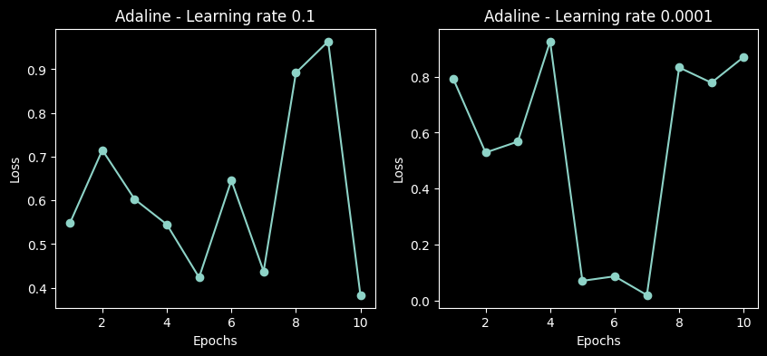
1行2列个子图

import numpy as np
import matplotlib.pyplot as plt

# 随机生成数据
np.random.seed(0)  # 确保结果可复现
losses_ada1 = np.random.rand(10)  # 学习率0.1的损失值
losses_ada2 = np.random.rand(10)  # 学习率0.0001的损失值

# 创建1行2列的子图
fig, ax = plt.subplots(nrows=1, ncols=2, figsize=(10, 4))

# 第一个子图：学习率0.1
ax[0].plot(range(1, len(losses_ada1) + 1), losses_ada1, marker='o')
ax[0].set_xlabel('Epochs')
ax[0].set_ylabel('Loss')
ax[0].set_title('Adaline - Learning rate 0.1')

# 第二个子图：学习率0.0001
ax[1].plot(range(1, len(losses_ada2) + 1), losses_ada2, marker='o')
ax[1].set_xlabel('Epochs')
ax[1].set_ylabel('Loss')
ax[1].set_title('Adaline - Learning rate 0.0001')

# 显示图形
plt.show()

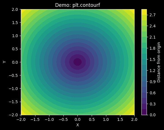
3.3、热力图

import numpy as np
import matplotlib.pyplot as plt

# 1. 创建 x 和 y 的一维坐标
x = np.linspace(-2, 2, 100)   # 从 -2 到 2，取 100 个点
y = np.linspace(-2, 2, 100)

# 2. 生成网格（每个点都有 (x, y) 坐标）
X, Y = np.meshgrid(x, y)

# 3. 定义一个函数：比如到原点的距离（形成圆形等高线）
Z = np.sqrt(X**2 + Y**2)   # 每个网格点到 (0,0) 的距离

# 4. 用 contourf 填充颜色
plt.contourf(X, Y, Z, levels=20, cmap='viridis')

# 5. 添加颜色条（可选）
plt.colorbar(label='Distance from origin')

# 6. 设置标题和坐标轴
plt.title('Demo: plt.contourf')
plt.xlabel('X')
plt.ylabel('Y')

# 7. 显示图形
plt.show()

4、scikit-learn

4.1、train_test_split（划分：训练集、测试集）

参数stratify：确保训练集和测试集中，每个类别样本的比例与划分前的数据集一致

from sklearn import datasets
import numpy as np
from sklearn.model_selection import train_test_split

iris = datasets.load_iris()
X = iris.data[:, [2, 3]]
y = iris.target

X_train, X_test, y_train, y_test = train_test_split(
    X, y, test_size=0.3, random_state=1, stratify=y)

print('Labels counts in y:', np.bincount(y))
print('Labels counts in y_train:', np.bincount(y_train))
print('Labels counts in y_test:', np.bincount(y_test))

Labels counts in y: [50 50 50]
Labels counts in y_train: [35 35 35]
Labels counts in y_test: [15 15 15]

4.2、StratifiedKFold（交叉验证，划分：训练集、测试集）

分层交叉验证，确保训练集和测试集中，每个类别样本的比例与划分前的数据集一致

from sklearn.model_selection import StratifiedKFold
from sklearn import datasets
import numpy as np

iris = datasets.load_iris()
X, y = iris.data, iris.target

skf = StratifiedKFold(n_splits=5, shuffle=True)  # 不打乱，便于观察

for fold, (train_idx, val_idx) in enumerate(skf.split(X, y), 1):
    print(f"Fold {fold}:")
    print("  训练集类别分布:", np.bincount(y[train_idx]))
    print("  验证集类别分布:", np.bincount(y[val_idx]))

Fold 1:
  训练集类别分布: [40 40 40]
  验证集类别分布: [10 10 10]
Fold 2:
  训练集类别分布: [40 40 40]
  验证集类别分布: [10 10 10]
Fold 3:
  训练集类别分布: [40 40 40]
  验证集类别分布: [10 10 10]
Fold 4:
  训练集类别分布: [40 40 40]
  验证集类别分布: [10 10 10]
Fold 5:
  训练集类别分布: [40 40 40]
  验证集类别分布: [10 10 10]

4.3、分类任务评估指标

指标	最适合场景	对不平衡敏感？	核心关注点
1. accuracy_score	类别平衡	极度敏感	整体预测正确率
2. precision_score	误报代价高（医疗误诊）	敏感	预测为正的样本中有多少是真的
3. recall_score	漏报代价高（如癌症筛查）	敏感	真实为正的样本中有多少被找出来了
4. f1_score	结合 precision 和 recall	敏感	P 和 R 的调和平均
5. kappa (Cohen’s Kappa)	类别不平衡、需排除随机一致性	✅ 鲁棒	超出随机猜测的一致性
6. AUC (ROC AUC)	模型需输出概率	✅ 中等（OvR 可能乐观）	模型区分正负类的能力（排序质量）

from sklearn.metrics import accuracy_score, precision_score, recall_score, f1_score, matthews_corrcoef, roc_auc_score

accuracy_score(y_test, y_pred)

# average=weighted: (prec_A * 900 + prec_B * 90 + prec_C * 10) / (900+90+10)
# average=macro: (prec_A + prec_B + prec_C) / 3
precision_score(y_true=y_test, y_pred=y_pred, average='weighted or macro')

recall_score(y_true=y_test, y_pred=y_pred, average='weighted or macro')

f1_score(y_true=y_test, y_pred=y_pred, average='weighted or macro')

kappa = cohen_kappa_score(y_test, y_pred)

# 假设 y_true 是真实标签，y_score 是模型预测的概率矩阵
# ovr（One-vs-Rest）：对每个类别单独计算 AUC，然后取平均。
auc_ovr = roc_auc_score(y_true, y_score, multi_class='ovr')
# ovo（One-vs-One）：两两类别之间计算 AUC，然后取平均。
auc_ovo = roc_auc_score(y_true, y_score, multi_class='ovo')

4.4、resample（降采样 / 过采样）

# 如果：y_imb==1的样本数量 > y_imb==0的样本数量，则以下代码对类别 0 过采样：
# 如果：y_imb==1的样本数量 < y_imb==0的样本数量，则以下代码对类别 0 降采样
from sklearn.utils import resample

print('Number of class 0 examples before:', X_imb[y_imb == 0].shape[0])

X_upsampled, y_upsampled = resample(X_imb[y_imb == 0],
                                    y_imb[y_imb == 0],
                                    replace=True,
                                    n_samples=X_imb[y_imb == 1].shape[0],
                                    random_state=123)

print('Number of class 0 examples after:', X_upsampled.shape[0])

4.5、计算MSE、MAE、R^2

1. 计算结果的大小受 y 的数值尺度影响
   • 均方根误差（MSE）
   • 平均绝对误差（MAE）
2. 计算结果的大小不受 y 的数值尺度影响，相当于MSE的标准化版本
   • 决定系数（R^2）

from sklearn.metrics import mean_squared_error, mean_absolute_error, r2_score

mean_squared_error(y_true, y_pred)

mean_absolute_error(y_true, y_pred)

r2_score(y_true, y_pred)

5、re（正则表达式）

5.1、优秀的学习资料

Google for education—Python 正则表达式

实践

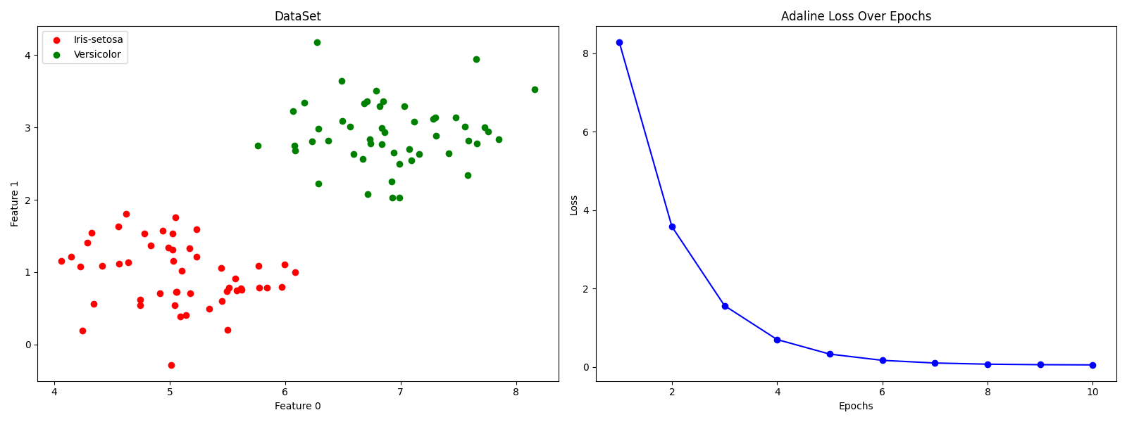
实践1：简单二分类

import numpy as np
import matplotlib.pyplot as plt

# load data
x1 = np.random.normal(loc=[5, 1], scale=[0.5,0.5], size=(50,2))
x2 = np.random.normal(loc=[7, 3], scale=[0.5,0.5], size=(50,2))
x = np.vstack((x1,x2))
y = np.hstack((np.zeros(50), np.ones(50)))

# plot data and loss in subplots
fig, (ax1, ax2) = plt.subplots(1, 2, figsize=(16, 6))

# scatter plot of the data points
ax1.scatter(x[:50, 0], x[:50, 1], color='red', marker='o', label='Iris-setosa')
ax1.scatter(x[50:100, 0], x[50:100, 1], color='green', marker='o', label='Versicolor')
ax1.set_xlabel('Feature 0')
ax1.set_ylabel('Feature 1')
ax1.set_title('DataSet')
ax1.legend(loc='upper left')

# model
class AdalineSGD:
    def __init__(self, epochs=10, lr=0.0001, seed=6):
        self.epochs = epochs
        self.lr = lr
        self.rgen = np.random.RandomState(seed)
        self.loss = []

    def init_params(self, shape):
        self.w_ = self.rgen.normal(loc=0.5, scale=0.05, size=shape)
        self.b_ = np.float_(0.0)

    def update_params(self, xi, yi):
        out = self.activate(self.net_input(xi))
        error = yi - out
        self.w_ += self.lr * error * xi
        self.b_ += self.lr * error
        return error ** 2

    def shuffle(self, x, y):
        r = self.rgen.permutation(len(y))
        return x[r], y[r]

    def fit(self, x, y):
        self.init_params(x.shape[1])
        x, y = self.shuffle(x, y)
        for _ in range(self.epochs):
            loss = []
            for xi, yi in zip(x, y):
                loss.append(self.update_params(xi, yi))
            self.loss.append(np.mean(loss))

    def net_input(self, x):
        return x @ self.w_ + self.b_

    def activate(self, x):
        return x

    def predict(self, x):
        return np.where(self.activate(self.net_input(x)) >= 0.5, 0, 1)

model = AdalineSGD()
model.fit(x, y)

# plot loss over epochs
ax2.plot(np.arange(1, len(model.loss) + 1), model.loss, color='blue', marker='o')
ax2.set_xlabel('Epochs')
ax2.set_ylabel('Loss')
ax2.set_title('Adaline Loss Over Epochs')

plt.tight_layout()
plt.show()