
DeepSeekMath的理解4——GRPO算法
文章目录
- 一、前言
- 二、DeepSeekMath
- 4. 强化学习
- 4.1. 群体相对策略优化(Group Relative Policy Optimization)
-
- 4.1.1. 从PPO到GRPO
- 4.2. DeepSeekMath-RL 的训练与评估
- 问题1:解释一下
- 问题2:完整故事
- 一、标准 KL 散度:衡量"你跑偏了多少"
- 二、PPO 的 KL 机制:图中"KL ⊕ r"的含义
- 三、GRPO 的 KL 机制:图中为什么 KL"单独走一路"
- 四、无偏估计器:公式 (4) 为什么长那样?
- 五、设计差异的根本原因总结
- 六、算法流程:结合伪代码图(Algorithm 1)
- 七、三种监督方式的直观解释
- 一句话总结整个故事
- 问题3:为什么这个无偏估计器"长这样"?
- 一、目标:我们要估计什么?
- 二、引入概率比值 r r r
- 三、核心推导(这次每一步都展开)
- 四、合并
- 五、数值验证(用 Python 直观展示)
- 一、我们要估计的目标
- 二、关键观察: r ( x ) r(x) r(x) 有一个"免费"的期望
- 三、构造无偏估计器
- 四、为什么这个形式更好?(数值性质)
- 五、和"标准 KL"的本质区别
- 六、一句话总结
- 问题4:推导公式解释
- 第一步:期望是什么?
- 第二步: r ( x ) r(x) r(x) 是什么?
- 第三步:把 r ( x ) r(x) r(x) 代入期望公式
- 第四步:抵消后剩下什么?
- 第五步:为什么 ∑ x π ref ( x ) = 1 \sum_x \pi_{\text{ref}}(x) = 1 ∑xπref(x)=1?
- 完整串起来
- 为什么这件事很巧妙?
一、前言
仅供参考,未经实验验证。这篇论文2024年发表的,看论文,那个时候DeepSeekMath就已经有过程监督这个概念了?
二、DeepSeekMath
论文标题: DeepSeekMath: Pushing the Limits of Mathematical Reasoning in Open Language Models
(DeepSeekMath:推动开放语言模型中数学推理的极限)
作者: Zhihong Shao, Peiyi Wang, Qihao Zhu, Runxin Xu, Junxiao Song, Mingchuan Zhang, Y.K. Li, Y. Wu, Daya Guo
机构: DeepSeek-AI(主导)、清华大学、北京大学
发表时间: 2024年2月6日(arXiv:2402.03300)
GitHub: https://github.com/deepseek-ai/DeepSeek-Math
4. 强化学习
4.1. 群体相对策略优化(Group Relative Policy Optimization)
4.1.1. 从PPO到GRPO
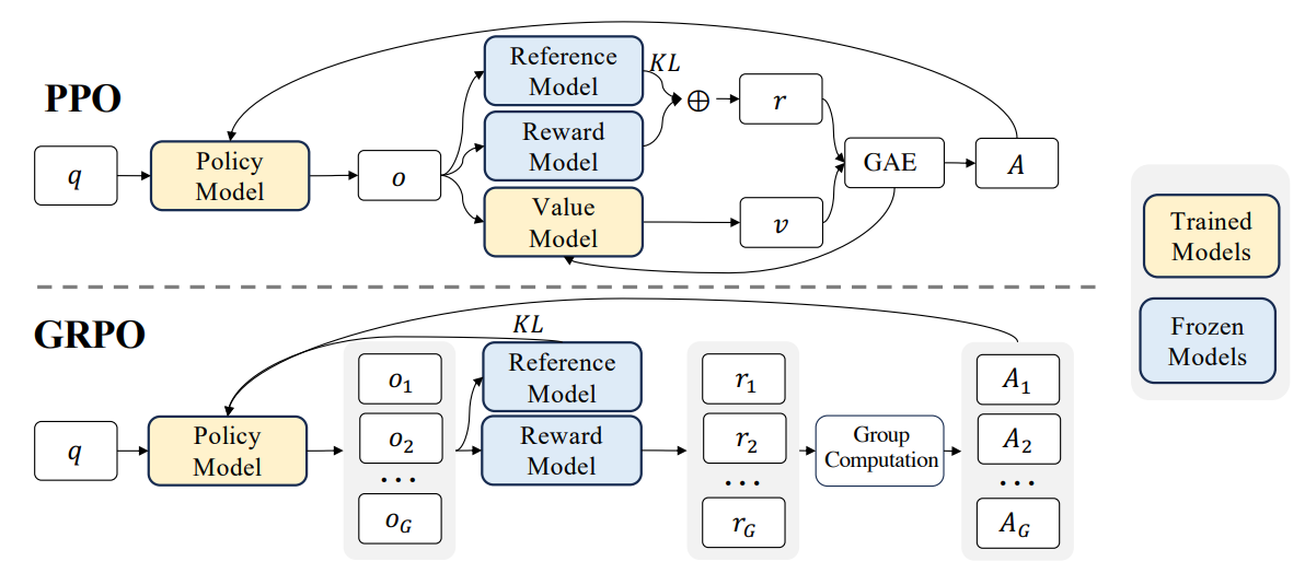
Figure 4 Demonstration of PPO and our GRPO. GRPO foregoes the value model, instead estimating the baseline from group scores, significantly reducing training resources.
图 4 PPO 和我们的 GRPO 的演示。GRPO 放弃了价值模型,而是从组分数估计基线,从而显著减少了训练资源。
As the value function employed in PPO is typically another model of comparable size as the policy model, it brings a substantial memory and computational burden. Additionally, during RL training, the value function is treated as a baseline in the calculation of the advantage for variance reduction.
由于PPO中使用的价值函数通常是与策略模型大小相当的另一个模型,因此会带来巨大的内存和计算负担。此外,在强化学习训练过程中,价值函数被视为基线,用于计算优势以减小方差。
While in the LLM context, usually only the last token is assigned a reward score by the reward model, which may complicate the training of a value function that is accurate at each token. To address this, as shown in Figure 4, we propose Group Relative Policy Optimization (GRPO), which obviates the need for additional value function approximation as in PPO, and instead uses the average reward of multiple sampled outputs, produced in response to the same question, as the baseline.
在LLM的上下文中,通常只有最后一个token会被奖励模型分配奖励分数,这可能会使每个token的价值函数训练变得复杂。为了解决这个问题,如图4所示,我们提出了分组相对策略优化(GRPO),它避免了像PPO那样额外的价值函数近似的需要,而是使用对同一问题产生的多个采样输出的平均奖励作为基线。
More specifically, for each question q q q , GRPO samples a group of outputs { o 1 , o 2 , … , o G } \{o_1, o_2, \dots, o_G\} {o1,o2,…,oG} from the old policy π θ o l d \pi_{\theta_{old}} πθold and then optimizes the policy model by maximizing the following objective:
更具体地说,对于每个问题 𝑞,GRPO 从旧策略 π θ o l d \pi_{\theta_{old}} πθold中采样一组输出 { o 1 , o 2 , … , o G } \{o_1, o_2, \dots, o_G\} {o1,o2,…,oG},然后通过最大化以下目标来优化策略模型:
J G R P O ( θ ) = E [ q ∼ P ( Q ) , { o i } i = 1 G ∼ π θ o l d ( O ∣ q ) ] 1 G ∑ i = 1 G 1 ∣ o i ∣ ∑ t = 1 ∣ o i ∣ { min [ π θ ( o i , t ∣ q , o i , < t ) π θ o l d ( o i , t ∣ q , o i , < t ) , A ^ i , t , clip ( π θ ( o i , t ∣ q , o i , < t ) π θ o l d ( o i , t ∣ q , o i , < t ) , 1 − ϵ , 1 + ϵ ) A ^ i , t ] − β D K L [ π θ ∣ ∣ π r e f ] } , ( 3 ) \begin{aligned} \mathcal{J}_{GRPO}(\theta) = & \mathbb{E}[q \sim P(Q), \{o_i\}_{i=1}^G \sim \pi_{\theta_{old}}(O|q)] \\ & \frac{1}{G} \sum_{i=1}^G \frac{1}{|o_i|} \sum_{t=1}^{|o_i|} \left\{ \min \left[ \frac{\pi_\theta(o_{i,t}|q, o_{i,<t})}{\pi_{\theta_{old}}(o_{i,t}|q, o_{i,<t})}, \hat{A}_{i,t}, \text{clip} \left( \frac{\pi_\theta(o_{i,t}|q, o_{i,<t})}{\pi_{\theta_{old}}(o_{i,t}|q, o_{i,<t})}, 1 - \epsilon, 1 + \epsilon \right) \hat{A}_{i,t} \right] - \beta \text{D}_{KL}[\pi_\theta || \pi_{ref}] \right\}, \quad (3) \end{aligned} JGRPO(θ)=E[q∼P(Q),{oi}i=1G∼πθold(O∣q)]G1i=1∑G∣oi∣1t=1∑∣oi∣{min[πθold(oi,t∣q,oi,<t)πθ(oi,t∣q,oi,<t),A^i,t,clip(πθold(oi,t∣q,oi,<t)πθ(oi,t∣q,oi,<t),1−ϵ,1+ϵ)A^i,t]−βDKL[πθ∣∣πref]},(3)
where ϵ \epsilon ϵ and β \beta β are hyper-parameters, and A ^ i , t \hat{A}_{i,t} A^i,t is the advantage calculated based on relative rewards of the outputs inside each group only, which will be detailed in the following subsections. The group relative way that GRPO leverages to calculate the advantages, aligns well with the comparative nature of rewards models, as reward models are typically trained on datasets of comparisons between outputs on the same question. Also note that, instead of adding KL penalty in the reward, GRPO regularizes by directly adding the KL divergence between the trained policy and the reference policy to the loss, avoiding complicating the calculation of A ^ i , t \hat{A}_{i,t} A^i,t .
其中 ϵ \epsilon ϵ 和 β \beta β 是超参数, A ^ i , t \hat{A}_{i,t} A^i,t 是基于组内输出的相对奖励计算出的优势值,具体细节将在后续小节中展开。GRPO 采用"组内相对"的方式来计算优势,这与奖励模型的比较本质高度契合——因为奖励模型通常是在"同一问题的不同输出之间的对比数据"上训练的。另外请注意,GRPO 没有将 KL 惩罚项加到奖励中,而是直接将训练策略与参考策略之间的 KL 散度加到损失函数上,从而避免了优势值 A ^ i , t \hat{A}_{i,t} A^i,t 的计算变得复杂。
And different from the KL penalty term used in (2), we estimate the KL divergence with the following unbiased estimator (Schulman, 2020):
与 (2) 式中使用的 KL 惩罚项不同,我们使用以下无偏估计器来估计 KL 散度(Schulman, 2020):
D KL [ π θ ∣ ∣ π ref ] = π ref ( o i , t ∣ q , o i , < t ) π θ ( o i , t ∣ q , o i , < t ) − log π ref ( o i , t ∣ q , o i , < t ) π θ ( o i , t ∣ q , o i , < t ) − 1 , ( 4 ) \mathbb{D}_{\text{KL}}[\pi_\theta || \pi_{\text{ref}}] = \frac{\pi_{\text{ref}}(o_{i,t} | q, o_{i,<t})}{\pi_\theta(o_{i,t} | q, o_{i,<t})} - \log \frac{\pi_{\text{ref}}(o_{i,t} | q, o_{i,<t})}{\pi_\theta(o_{i,t} | q, o_{i,<t})} - 1, \quad (4) DKL[πθ∣∣πref]=πθ(oi,t∣q,oi,<t)πref(oi,t∣q,oi,<t)−logπθ(oi,t∣q,oi,<t)πref(oi,t∣q,oi,<t)−1,(4)
which is guaranteed to be positive.
该估计器保证始终为非负值。
4.1.2. 基于 GRPO 的结果监督强化学习(Outcome Supervision RL with GRPO)
Formally, for each question q q q , a group of outputs { o 1 , o 2 , … , o G } \{o_1, o_2, \dots, o_G\} {o1,o2,…,oG} are sampled from the old policy model π θ old \pi_{\theta_{\text{old}}} πθold . A reward model is then used to score the outputs, yielding G G G rewards r = { r 1 , r 2 , … , r G } \mathbf{r} = \{r_1, r_2, \dots, r_G\} r={r1,r2,…,rG} correspondingly. Subsequently, these rewards are normalized by subtracting the group average and dividing by the group standard deviation. Outcome supervision provides the normalized reward at the end of each output o i o_i oi and sets the advantages A ^ i , t \hat{A}_{i,t} A^i,t of all tokens in the output as the normalized reward, i.e., A ^ i , t = r ~ i = r i − mean ( r ) std ( r ) \hat{A}_{i,t} = \tilde{r}_i = \frac{r_i - \text{mean}(\mathbf{r})}{\text{std}(\mathbf{r})} A^i,t=r~i=std(r)ri−mean(r) , and then optimizes the policy by maximizing the objective defined in equation (3).
形式上,对于每个问题 q q q,从旧策略模型 π θ old \pi_{\theta_{\text{old}}} πθold 中采样一组输出 { o 1 , o 2 , … , o G } \{o_1, o_2, \dots, o_G\} {o1,o2,…,oG}。然后使用奖励模型对这些输出打分,得到对应的 G G G 个奖励 r = { r 1 , r 2 , … , r G } \mathbf{r} = \{r_1, r_2, \dots, r_G\} r={r1,r2,…,rG}。随后,这些奖励通过减去组内平均值并除以组内标准差进行归一化。结果监督在每个输出 o i o_i oi 的末尾提供归一化奖励,并将输出中所有 token 的优势值 A ^ i , t \hat{A}_{i,t} A^i,t 设为该归一化奖励,即 A ^ i , t = r ~ i = r i − mean ( r ) std ( r ) \hat{A}_{i,t} = \tilde{r}_i = \frac{r_i - \text{mean}(\mathbf{r})}{\text{std}(\mathbf{r})} A^i,t=r~i=std(r)ri−mean(r),然后通过最大化方程 (3) 中定义的目标来优化策略。
4.1.3. 基于 GRPO 的过程监督强化学习(Process Supervision RL with GRPO)
Outcome supervision only provides a reward at the end of each output, which may not be sufficient and efficient to supervise the policy in complex mathematical tasks. Following Wang et al. (2023b), we also explore process supervision, which provides a reward at the end of each reasoning step. Formally, given the question q q q and G G G sampled outputs { o 1 , o 2 , … , o G } \{o_1, o_2, \dots, o_G\} {o1,o2,…,oG} , a process reward model is used to score each step of the outputs, yielding corresponding rewards: R = { { r 1 index ( 1 ) , … , r K 1 index ( K 1 ) } , … , { r G index ( 1 ) , … , r G index ( K G ) } } \mathbf{R} = \{\{r_1^{\text{index}(1)}, \dots, r_{K_1}^{\text{index}(K_1)}\}, \dots, \{r_G^{\text{index}(1)}, \dots, r_G^{\text{index}(K_G)}\}\} R={{r1index(1),…,rK1index(K1)},…,{rGindex(1),…,rGindex(KG)}} , where index ( j ) \text{index}(j) index(j) is the end token index of the j j j -th step, and K i K_i Ki is the total number of steps in the i i i -th output. We also normalize these rewards with the average and the standard deviation, i.e., r ~ i index ( j ) = r i index ( j ) − mean ( R ) std ( R ) \tilde{r}_i^{\text{index}(j)} = \frac{r_i^{\text{index}(j)} - \text{mean}(\mathbf{R})}{\text{std}(\mathbf{R})} r~iindex(j)=std(R)riindex(j)−mean(R) . Subsequently, the process supervision calculates the advantage of each token as the sum of the normalized rewards from the following steps, i.e., A ^ i , t = ∑ index ( j ) ≥ t r ~ i index ( j ) \hat{A}_{i,t} = \sum_{\text{index}(j) \geq t} \tilde{r}_i^{\text{index}(j)} A^i,t=∑index(j)≥tr~iindex(j) , and then optimizes the policy by maximizing the objective defined in equation (3).
结果监督只在每个输出的末尾提供一个奖励,这对于复杂数学任务中的策略监督来说可能不够充分和高效。遵循 Wang 等人 (2023b) 的方法,我们也探索了过程监督,即在每个推理步骤的末尾提供奖励。形式上,给定问题 q q q 和 G G G 个采样输出 { o 1 , o 2 , … , o G } \{o_1, o_2, \dots, o_G\} {o1,o2,…,oG},使用过程奖励模型对输出的每一步进行打分,得到对应的奖励: R = { { r 1 index ( 1 ) , … , r K 1 index ( K 1 ) } , … , { r G index ( 1 ) , … , r G index ( K G ) } } \mathbf{R} = \{\{r_1^{\text{index}(1)}, \dots, r_{K_1}^{\text{index}(K_1)}\}, \dots, \{r_G^{\text{index}(1)}, \dots, r_G^{\text{index}(K_G)}\}\} R={{r1index(1),…,rK1index(K1)},…,{rGindex(1),…,rGindex(KG)}},其中 index ( j ) \text{index}(j) index(j) 是第 j j j 个步骤的结束 token 索引, K i K_i Ki 是第 i i i 个输出的总步数。我们同样用平均值和标准差对这些奖励进行归一化,即 r ~ i index ( j ) = r i index ( j ) − mean ( R ) std ( R ) \tilde{r}_i^{\text{index}(j)} = \frac{r_i^{\text{index}(j)} - \text{mean}(\mathbf{R})}{\text{std}(\mathbf{R})} r~iindex(j)=std(R)riindex(j)−mean(R)。随后,过程监督将每个 token 的优势值计算为后续步骤归一化奖励的累加,即 A ^ i , t = ∑ index ( j ) ≥ t r ~ i index ( j ) \hat{A}_{i,t} = \sum_{\text{index}(j) \geq t} \tilde{r}_i^{\text{index}(j)} A^i,t=∑index(j)≥tr~iindex(j),然后通过最大化方程 (3) 中定义的目标来优化策略。
4.1.4. 基于GRPO的迭代强化学习(Iterative RL with GRPO)
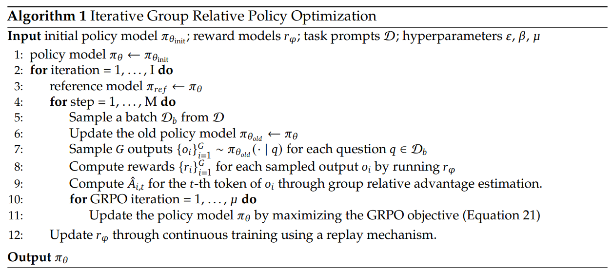
As the reinforcement learning training process progresses, the old reward model may not be sufficient to supervise the current policy model. Therefore, we also explore the iterative RL with GRPO. As shown in Algorithm 1, in iterative GRPO, we generate new training sets for the reward model based on the sampling results from the policy model and continually train the old reward model using a replay mechanism that incorporates 10% of historical data.Then, we set the reference model as the policy model, and continually train the policy model with the new reward model.
随着强化学习训练过程的推进,旧的奖励模型可能不足以监督当前的策略模型。因此,我们还探索了结合GRPO的迭代强化学习。如算法1所示,在迭代GRPO中,我们根据策略模型的采样结果生成新的奖励模型训练集,并通过包含10%历史数据的回放机制持续训练旧奖励模型。然后,我们将参考模型设置为策略模型,并使用新的奖励模型持续训练策略模型。
4.2. DeepSeekMath-RL 的训练与评估
We conduct RL based on DeepSeekMath-Instruct 7B. The training data of RL are chain-ofthought-format questions related to GSM8K and MATH from the SFT data, which consists of around 144K questions. We exclude other SFT questions to investigate the impact of RL on benchmarks that lack data throughout the RL phase.
我们基于DeepSeekMath-Instruct 7B进行强化学习。强化学习的训练数据为SFT数据中与GSM8K和MATH相关的思维链格式问题,共计约144K个问题。我们排除了其他的SFT问题,以探究强化学习在强化学习阶段缺乏数据基准上的影响。
We construct the training set of reward models following (Wang et al., 2023b). We train our initial reward model based on the DeepSeekMath-Base 7B with a learning rate of 2e-5. For GRPO, we set the learning rate of the policy model as 1e-6.
我们按照 (Wang et al., 2023b) 构建奖励模型训练集。我们基于 DeepSeekMath-Base 7B 训练初始奖励模型,学习率为 2e-5。对于 GRPO,我们将策略模型的学习率设置为 1e-6。
The KL coefficient is 0.04. For each question, we sample 64 outputs. The max length is set to 1024, and the training batch size is 1024. The policy model only has a single update following each exploration stage. We evaluate DeepSeekMath-RL 7B on benchmarks following DeepSeekMath-Instruct 7B.
KL散度系数为0.04。对于每个问题,我们采样64个输出。最大长度设置为1024,训练批次大小为1024。策略模型在每次探索阶段后仅进行一次更新。我们在遵循DeepSeekMath-Instruct 7B的基准上评估DeepSeekMath-RL 7B。
For DeepSeekMath-RL 7B, GSM8K and MATH with chain-of-thought reasoning can be regarded as in-domain tasks and all the other benchmarks can be regarded as out-of-domain tasks.
对于DeepSeekMath-RL 7B,具有思维链推理的GSM8K和MATH可以被视为域内任务,而所有其他基准测试可以被视为域外任务。
Table 5 demonstrates the performance of open- and closed-source models with both chainof-thought and tool-integrated reasoning on English and Chinese benchmarks. We find that:
- DeepSeekMath-RL 7B attains accuracies of 88.2% and 51.7% on GSM8K and MATH, respectively, utilizing chain-of-thought reasoning. This performance surpasses that of all open-source models in the 7B to 70B range, as well as the majority of closed-source models.
- Crucially, DeepSeekMath-RL 7B is only trained on chain-of-thought-format instruction tuning data of GSM8K and MATH, starting from DeepSeekMath-Instruct 7B.
表 5 展示了在英文和中文基准测试上,结合了思维链和工具集成推理的开源与闭源模型的性能。我们发现: - DeepSeekMath-RL 7B 在 GSM8K 和 MATH 数据集上分别达到了 88.2% 和 51.7% 的准确率,使用了思维链推理。这一性能超过了 7B 到 70B 范围内所有开源模型以及大多数闭源模型的性能。
- 至关重要的是,DeepSeekMath-RL 7B 仅在 GSM8K 和 MATH 的思维链格式指令调优数据上进行了训练,该模型是从 DeepSeekMath-Instruct 7B 开始训练的。
Despite the constrained scope of its training data, it outperforms DeepSeekMath-Instruct 7B across all evaluation metrics, showcasing the effectiveness of reinforcement learning.
尽管其训练数据的范围有限,但它在所有评估指标上均优于DeepSeekMath-Instruct 7B,这表明了强化学习的有效性。
问题1:解释一下
1. GRPO 要解决的核心痛点
PPO 的问题:在标准 PPO 中,你需要同时训练两个大模型——
- 策略模型(Policy):负责生成回答
- 价值模型(Value):负责评估"当前状态有多好"
价值模型通常和策略模型一样大,内存和计算开销翻倍。更麻烦的是,在 LLM 场景中,奖励模型通常只给回答的最后一个 token 打分,这让价值模型很难学会"每个中间 token 值多少分",训练困难且不准。
GRPO 的解法:干脆不要价值模型了!对同一个问题,让旧策略生成一组回答(比如 64 个),用这 64 个回答的平均奖励作为基线(baseline)。某个回答比平均好,就鼓励;比平均差,就抑制。
2. 公式 (3) 的直观拆解
J G R P O ( θ ) = E [ 1 G ∑ i = 1 G 1 ∣ o i ∣ ∑ t = 1 ∣ o i ∣ { min [ ratio ⋅ A ^ , clip ( ratio ) ⋅ A ^ ] − β ⋅ D K L } ] \mathcal{J}_{GRPO}(\theta) = \mathbb{E}\left[\frac{1}{G} \sum_{i=1}^G \frac{1}{|o_i|} \sum_{t=1}^{|o_i|} \left\{ \min\left[ \text{ratio} \cdot \hat{A}, \text{clip}(\text{ratio}) \cdot \hat{A} \right] - \beta \cdot D_{KL} \right\}\right] JGRPO(θ)=E G1i=1∑G∣oi∣1t=1∑∣oi∣{min[ratio⋅A^,clip(ratio)⋅A^]−β⋅DKL}
| 符号 | 含义 | 通俗理解 |
|---|---|---|
| G G G | 组大小 | 同一个问题生成 64 个回答 |
| ratio \text{ratio} ratio | π θ π θ o l d \frac{\pi_\theta}{\pi_{\theta_{old}}} πθoldπθ | 新策略生成这个 token 的概率 / 旧策略生成它的概率 |
| A ^ i , t \hat{A}_{i,t} A^i,t | 优势值 | 这个回答(或这个 token)比组内平均好多少 |
| min [ … ] \min[\dots] min[…] | 裁剪目标 | 防止新策略变化太快(PPO 的经典做法) |
| D K L D_{KL} DKL | KL 散度 | 惩罚新策略偏离参考模型(SFT 模型)太远 |
| β \beta β | KL 系数 | 控制"别太放飞自我"的力度 |
一句话:对每个 token,看新策略比旧策略更愿意生成它的程度(ratio),乘以这个回答的优势值,但限制变化幅度,同时惩罚偏离原始 SFT 模型太远。
3. 结果监督 vs 过程监督
结果监督(Outcome):
- 只关心最终答案对不对
- 64 个回答 → 64 个分数 → 归一化 → 每个回答里的所有 token 共享同一个优势值
- 好比老师只根据期末考试成绩给学生打分,平时作业不管
过程监督(Process):
- 每个推理步骤结束都打分(比如解数学题,每算一步都给分)
- 某个 token 的优势值 = 它所在步骤及之后所有步骤的分数之和
- 好比老师每做一步题都批改,前面的 token 要为后面的正确步骤"负责"
- 好处:复杂任务中,模型能知道"哪一步走错了",训练信号更精细
4. 公式 (4) 的 KL 散度估计器
标准 KL 散度计算需要积分/期望,实际实现麻烦。这里用了一个无偏估计器:
D K L = π r e f π θ − log π r e f π θ − 1 D_{KL} = \frac{\pi_{ref}}{\pi_\theta} - \log\frac{\pi_{ref}}{\pi_\theta} - 1 DKL=πθπref−logπθπref−1
令 r = π r e f π θ r = \frac{\pi_{ref}}{\pi_\theta} r=πθπref,则 D K L = r − log r − 1 D_{KL} = r - \log r - 1 DKL=r−logr−1。
- 当新旧策略完全一致时, r = 1 r=1 r=1, D K L = 0 D_{KL} = 0 DKL=0
- 当 r ≠ 1 r \neq 1 r=1 时,这个值恒大于 0
- 不需要额外采样估计,直接用当前 token 的概率比就能算,数值稳定
5. 迭代强化学习(Iterative RL)
问题:策略模型越变越强,旧的奖励模型可能"看不懂"新策略生成的花样,打分不准。
做法:
- 用当前策略模型生成新数据,扩充奖励模型训练集
- 保留 10% 历史数据(防止遗忘),重新训练奖励模型
- 把参考模型更新为当前策略模型,继续 RL 训练
本质:奖励模型和策略模型"交替升级",避免一方掉队。
6. 实验设置的含义
| 参数 | 数值 | 含义 |
|---|---|---|
| 学习率 1e-6 | 很小 | 策略模型已经经过 SFT,只微调,步子要小 |
| KL 系数 0.04 | 中等 | 允许一定探索,但不能偏离 SFT 模型太远 |
| 每组 64 个输出 | 较大 | 组越大,基线估计越稳定,但计算量越大 |
| Batch 1024 | — | 并行处理 1024 个问题,每个问题 64 个回答 |
| 每次探索只更新一次 | 保守 | 生成完一批数据,策略只走一步,稳定性优先 |
总结一句话
GRPO = PPO 去掉价值模型 + 用组内相对奖励算优势 + KL 直接放损失里 + 支持过程/结果/迭代三种监督方式。它用"同组比较"替代"绝对评估",大幅降低了 RL 训练的资源消耗,同时让奖励信号更贴合奖励模型的比较本质。
问题2:完整故事
把整个故事说完整,比如算法是怎么运行的,标准KL散度是怎么样的,PPO的KL散度是怎么样的,为什么图中显示PPO的KL散度是从参考模型和奖励模型出来然后加起来得到r的,然后为什么GRPO的KL散度只是从奖励模型指向了策略模型,无偏估计器的公式为什么长那样?造成这些设计上的不同的原因是什么?结果监督、过程监督、迭代的强化学习,这些直观的解释是怎么样的?
我把 GRPO 的完整故事从头到尾串一遍——从标准 KL 散度是什么,到PPO 为什么那样画,再到GRPO 为什么这样改,最后到算法怎么跑起来。
一、标准 KL 散度:衡量"你跑偏了多少"
标准 KL 散度(Kullback-Leibler Divergence)是衡量两个概率分布差异的指标:
KL ( π θ ∥ π ref ) = E x ∼ π θ [ log π θ ( x ) π ref ( x ) ] \text{KL}(\pi_\theta \| \pi_{\text{ref}}) = \mathbb{E}_{x \sim \pi_\theta}\left[\log\frac{\pi_\theta(x)}{\pi_{\text{ref}}(x)}\right] KL(πθ∥πref)=Ex∼πθ[logπref(x)πθ(x)]
- 直观:如果新策略 π θ \pi_\theta πθ 和参考策略(通常是 SFT 后的模型) π ref \pi_{\text{ref}} πref 生成每个 token 的概率差不多,KL 就接近 0;跑越远,KL 越大。
- 性质:非负,只有当两个分布完全一样时才为 0。
二、PPO 的 KL 机制:图中"KL ⊕ r"的含义
看第一张图的上半部分(PPO):
Reference Model ──┐
                 ├──⊕──→ r ──┐
Reward Model ────┘           ├──→ GAE ──→ A
Value Model ─────────────→ v ─┘
这里发生了什么?
- Reward Model 给回答打一个原始分 r raw r_{\text{raw}} rraw
- Reference Model 计算当前策略和原始策略的 KL 散度
- 两者通过 ⊕(相加)合并: r = r raw − β ⋅ KL r = r_{\text{raw}} - \beta \cdot \text{KL} r=rraw−β⋅KL
- 也就是说,KL 惩罚直接扣在了奖励上
- 这个被 KL"污染"过的奖励 r r r,再和 Value Model 估计的价值 v v v 一起送进 GAE(广义优势估计),算出优势值 A A A
这样做的代价:
- 你需要同时维护一个和策略模型一样大的 Value Model,内存翻倍
- 在 LLM 场景中,奖励模型通常只给回答的最后一个 token 打分,导致 Value Model 很难学会"中间每个 token 值多少"
- 更关键的是:KL 参与了 GAE 计算,优势值 A A A 的计算因此变得复杂,耦合度高
三、GRPO 的 KL 机制:图中为什么 KL"单独走一路"
看第一张图的下半部分(GRPO):
Policy Model ──→ {o₁, o₂, ..., o_G}
                    ↓
Reference Model ─────→ KL(单独指向策略模型)
                    ↓
Reward Model ──→ {r₁, r₂, ..., r_G} ──→ Group Computation ──→ {A₁, A₂, ..., A_G}
关键区别:
| 设计 | PPO | GRPO |
|---|---|---|
| 基线(Baseline) | Value Model 估计 | 组内平均奖励 |
| KL 位置 | 塞进奖励里: r = r raw − β ⋅ KL r = r_{\text{raw}} - \beta \cdot \text{KL} r=rraw−β⋅KL | 直接加到损失函数里,和奖励分开 |
| 优势计算 | GAE 需要 r r r 和 v v v | Group Computation 只看组内相对奖励 |
为什么 GRPO 敢这样改?
因为 GRPO 抛弃了 Value Model,改用**"组内相对"算优势:对同一个问题生成 G G G 个回答,用这 G G G 个回答的平均奖励**作为基线。既然不需要 Value Model,也就不需要 GAE 那套复杂的时序差分计算。
- 如果 KL 还像 PPO 一样放在奖励里,那 Group Computation 算优势时就要处理 KL,反而把简单的东西搞复杂了
- 所以 GRPO 直接把 KL 散度项从奖励中解耦,单独放在最终的损失函数中:
Loss = − J GRPO + β ⋅ D KL \text{Loss} = -\mathcal{J}_{\text{GRPO}} + \beta \cdot \mathbb{D}_{\text{KL}} Loss=−JGRPO+β⋅DKL
图中 KL 单独指向策略模型的含义:KL 只作为正则项直接约束策略更新,不参与优势值 A A A 的计算流程,也不经过 Group Computation。
四、无偏估计器:公式 (4) 为什么长那样?
公式 (4) 给出:
D KL = π ref π θ − log π ref π θ − 1 \mathbb{D}_{\text{KL}} = \frac{\pi_{\text{ref}}}{\pi_\theta} - \log\frac{\pi_{\text{ref}}}{\pi_\theta} - 1 DKL=πθπref−logπθπref−1
令 r = π ref ( o i , t ) π θ ( o i , t ) r = \frac{\pi_{\text{ref}}(o_{i,t})}{\pi_\theta(o_{i,t})} r=πθ(oi,t)πref(oi,t),则 D KL = r − log r − 1 \mathbb{D}_{\text{KL}} = r - \log r - 1 DKL=r−logr−1
为什么这个无偏估计器"长这样"?核心推导只有三行:
-
在期望意义下, E x ∼ π θ [ r ] = E x ∼ π θ [ π ref ( x ) π θ ( x ) ] = ∑ x π θ ( x ) ⋅ π ref ( x ) π θ ( x ) = ∑ x π ref ( x ) = 1 \mathbb{E}_{x \sim \pi_\theta}[r] = \mathbb{E}_{x \sim \pi_\theta}\left[\frac{\pi_{\text{ref}}(x)}{\pi_\theta(x)}\right] = \sum_x \pi_\theta(x) \cdot \frac{\pi_{\text{ref}}(x)}{\pi_\theta(x)} = \sum_x \pi_{\text{ref}}(x) = 1 Ex∼πθ[r]=Ex∼πθ[πθ(x)πref(x)]=∑xπθ(x)⋅πθ(x)πref(x)=∑xπref(x)=1
-
标准 KL 散度: KL ( π θ ∥ π ref ) = E x ∼ π θ [ log π θ ( x ) π ref ( x ) ] = E [ − log r ] \text{KL}(\pi_\theta \| \pi_{\text{ref}}) = \mathbb{E}_{x \sim \pi_\theta}\left[\log\frac{\pi_\theta(x)}{\pi_{\text{ref}}(x)}\right] = \mathbb{E}[-\log r] KL(πθ∥πref)=Ex∼πθ[logπref(x)πθ(x)]=E[−logr]
-
所以:
E [ r − log r − 1 ] = E [ r ] ⏟ = 1 − E [ log r ] − 1 = − E [ log r ] = KL ( π θ ∥ π ref ) \mathbb{E}[r - \log r - 1] = \underbrace{\mathbb{E}[r]}_{=1} - \mathbb{E}[\log r] - 1 = -\mathbb{E}[\log r] = \text{KL}(\pi_\theta \| \pi_{\text{ref}}) E[r−logr−1]==1 E[r]−E[logr]−1=−E[logr]=KL(πθ∥πref)
结论:对单个 token 取 r − log r − 1 r - \log r - 1 r−logr−1,它的期望精确等于 KL 散度,因此是无偏估计。
为什么用它而不是标准 KL?
- 数值稳定: r − log r − 1 ≥ 0 r - \log r - 1 \geq 0 r−logr−1≥0 对所有 r > 0 r > 0 r>0 恒成立(你可以画一下 f ( x ) = x − log x − 1 f(x)=x-\log x-1 f(x)=x−logx−1,在 x = 1 x=1 x=1 处取最小值 0),天然满足 KL 非负性
- 实现简单:不需要额外采样,直接用当前 batch 中 π ref \pi_{\text{ref}} πref 和 π θ \pi_\theta πθ 的概率比就能算
五、设计差异的根本原因总结
| 问题 | PPO 的困境 | GRPO 的解法 |
|---|---|---|
| 价值函数难训 | LLM 只有最后 token 有奖励,中间 token 的价值难以估计 | 干脆不要 Value Model,用组内平均做基线 |
| 奖励模型本质 | 奖励模型训练数据是"同一问题的对比",PPO 却用绝对值估计 | GRPO 的组内相对计算天然匹配奖励模型的比较本质 |
| KL 与优势耦合 | KL 在奖励里,GAE 计算必须考虑它,复杂且容易不稳定 | KL 直接放损失里,优势计算保持干净 |
| 内存开销 | Policy + Value + Reference + Reward,四个大模型 | Policy + Reference + Reward,省掉一个 Value Model |
六、算法流程:结合伪代码图(Algorithm 1)
输入:初始策略 π_θ_init,奖励模型 r_φ,问题集 D,超参数 ε, β, μ

1.  策略模型 π_θ ← π_θ_init
2.  外层循环(迭代轮数 iteration = 1, ..., I):
3.      参考模型 π_ref ← π_θ        ← 每轮开始,把参考模型更新为当前策略
4.      内层循环(训练步 step = 1, ..., M):
5.          从 D 中采样一个 batch D_b
6.          旧策略 π_θ_old ← π_θ    ← 固定旧策略用于采样
7.          对每个问题 q ∈ D_b:
8.              用旧策略采样 G 个回答 {o₁, ..., o_G}
9.              奖励模型打分 → {r₁, ..., r_G}
10.             组内计算优势 Â_{i,t}
11.         内层 GRPO 更新(迭代 μ 次):
12.             最大化 GRPO 目标函数(公式 3)更新策略 π_θ
13.     用回放机制(10% 历史数据)更新奖励模型 r_φ

输出:π_θ
关键步骤的直观解释:
- 第 3 行:参考模型每轮都更新为当前策略。这意味着 KL 惩罚的"锚点"是动态前进的,不是永远固定在最初的 SFT 模型。
- 第 6 行:采样和更新分离。先生成一批数据,再在这批数据上更新策略,避免"边生成边更新"导致的数据分布漂移。
- 第 10 行:Group Computation 就是"组内归一化"——减去组内均值,除以组内标准差。
- 第 12 行: μ \mu μ 次迭代意味着同一批数据会被策略模型反复学习多次(类似 PPO 的 epoch)。
- 第 13 行:奖励模型也要跟着进化,否则策略变强了,奖励模型可能"看不懂"新策略的玩法。
七、三种监督方式的直观解释
1. 结果监督(Outcome Supervision)
- 像期末考试:只看你最终答案对不对,不管中间怎么想的
- 实现:64 个回答 → 64 个总分 → 归一化 → 每个回答里的所有 token 共享同一个优势值
- 局限:如果答案错了,模型不知道是哪一步推错了
2. 过程监督(Process Supervision)
- 像老师逐步批改:解数学题,每写一步都打分
- 实现:每个推理步骤结束都有一个奖励,某个 token 的优势 = 它所在步骤及之后所有步骤的奖励之和
- 好处:前面的 token 要为后面的正确步骤"负责",训练信号更精细,适合复杂推理
3. 迭代强化学习(Iterative RL)
- 像师生共同进步:学生(策略)变聪明了,老师(奖励模型)也得跟着学,否则老师看不懂学生的创新解法
- 实现:用当前策略生成新数据,混合 10% 旧数据重新训练奖励模型,然后参考模型也更新为当前策略,继续下一轮
一句话总结整个故事
PPO 用"价值模型"估计每个状态值多少钱,再把 KL 塞进奖励里一起算优势,结果在 LLM 场景下又重又难训;GRPO 干脆扔掉价值模型,对同一个问题生成一堆回答互相比较算优势,把 KL 单独拎出来直接加在损失上,用 Schulman 的无偏估计器稳定计算,最终实现了更轻量、更贴合奖励模型本质的强化学习。
问题3:为什么这个无偏估计器"长这样"?
为什么这个无偏估计器"长这样"?核心推导只有三行。这部分没看懂
我把它拆成数学推导和数值验证两部分,一步步讲清楚。
一、目标:我们要估计什么?
标准 KL 散度的定义是:
KL ( π θ ∥ π ref ) = E x ∼ π θ [ log π θ ( x ) π ref ( x ) ] \text{KL}(\pi_\theta \| \pi_{\text{ref}}) = \mathbb{E}_{x \sim \pi_\theta}\left[\log\frac{\pi_\theta(x)}{\pi_{\text{ref}}(x)}\right] KL(πθ∥πref)=Ex∼πθ[logπref(x)πθ(x)]
也就是说:从当前策略 π θ \pi_\theta πθ 中采样,计算 log π θ π ref \log\frac{\pi_\theta}{\pi_{\text{ref}}} logπrefπθ,求期望。
二、引入概率比值 r r r
令:
r ( x ) = π ref ( x ) π θ ( x ) r(x) = \frac{\pi_{\text{ref}}(x)}{\pi_\theta(x)} r(x)=πθ(x)πref(x)
那么标准 KL 可以改写成:
KL = E x ∼ π θ [ log 1 r ( x ) ] = E x ∼ π θ [ − log r ( x ) ] \text{KL} = \mathbb{E}_{x \sim \pi_\theta}\left[\log\frac{1}{r(x)}\right] = \mathbb{E}_{x \sim \pi_\theta}\left[-\log r(x)\right] KL=Ex∼πθ[logr(x)1]=Ex∼πθ[−logr(x)]
三、核心推导(这次每一步都展开)
我们要证明: r − log r − 1 r - \log r - 1 r−logr−1 的期望 = KL
把 f ( r ) = r − log r − 1 f(r) = r - \log r - 1 f(r)=r−logr−1 拆开求期望:
E x ∼ π θ [ f ( r ) ] = E [ r ] ⏟ 第①项 − E [ log r ] ⏟ 第②项 − E [ 1 ] ⏟ 第③项 \mathbb{E}_{x \sim \pi_\theta}[f(r)] = \underbrace{\mathbb{E}[r]}_{\text{第①项}} - \underbrace{\mathbb{E}[\log r]}_{\text{第②项}} - \underbrace{\mathbb{E}[1]}_{\text{第③项}} Ex∼πθ[f(r)]=第①项 E[r]−第②项 E[logr]−第③项 E[1]
第①项: E x ∼ π θ [ r ] \mathbb{E}_{x \sim \pi_\theta}[r] Ex∼πθ[r]
E x ∼ π θ [ π ref ( x ) π θ ( x ) ] = ∑ x π θ ( x ) ⋅ π ref ( x ) π θ ( x ) = ∑ x π ref ( x ) = 1 \mathbb{E}_{x \sim \pi_\theta}\left[\frac{\pi_{\text{ref}}(x)}{\pi_\theta(x)}\right] = \sum_x \pi_\theta(x) \cdot \frac{\pi_{\text{ref}}(x)}{\pi_\theta(x)} = \sum_x \pi_{\text{ref}}(x) = 1 Ex∼πθ[πθ(x)πref(x)]=x∑πθ(x)⋅πθ(x)πref(x)=x∑πref(x)=1
关键: π θ ( x ) \pi_\theta(x) πθ(x) 和分母抵消,剩下 π ref ( x ) \pi_{\text{ref}}(x) πref(x) 的求和,而概率分布求和恒为 1。
第②项: E x ∼ π θ [ log r ] \mathbb{E}_{x \sim \pi_\theta}[\log r] Ex∼πθ[logr]
E [ log π ref π θ ] = − E [ log π θ π ref ] = − KL ( π θ ∥ π ref ) \mathbb{E}\left[\log\frac{\pi_{\text{ref}}}{\pi_\theta}\right] = -\mathbb{E}\left[\log\frac{\pi_\theta}{\pi_{\text{ref}}}\right] = -\text{KL}(\pi_\theta \| \pi_{\text{ref}}) E[logπθπref]=−E[logπrefπθ]=−KL(πθ∥πref)
第③项: E [ 1 ] = 1 \mathbb{E}[1] = 1 E[1]=1
四、合并
E [ r − log r − 1 ] = 1 − ( − KL ) − 1 = KL ( π θ ∥ π ref ) \mathbb{E}[r - \log r - 1] = 1 - (-\text{KL}) - 1 = \text{KL}(\pi_\theta \| \pi_{\text{ref}}) E[r−logr−1]=1−(−KL)−1=KL(πθ∥πref)
证毕。 这就是为什么它被称为"无偏估计器"——对单个样本计算 r − log r − 1 r - \log r - 1 r−logr−1,取平均后的期望精确等于 KL 散度。
五、数值验证(用 Python 直观展示)
我用一个具体的离散分布来验证这个等式,同时画出 f ( r ) = r − log r − 1 f(r) = r - \log r - 1 f(r)=r−logr−1 的图像,让你看到它为什么恒非负。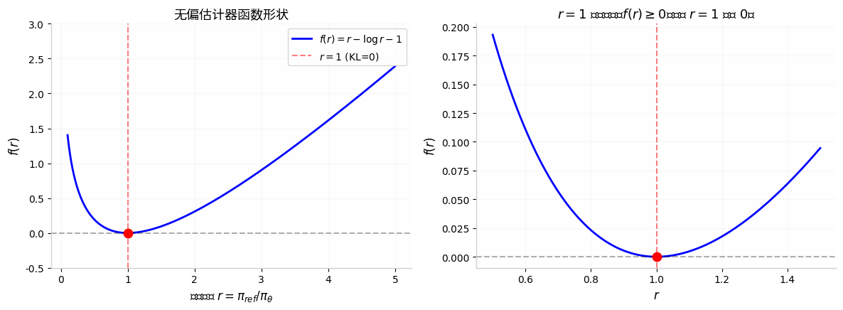
从代码验证可以看到,标准 KL 散度 = 0.028534,无偏估计器的期望 = 0.028534,两者差异只有 1.73 × 10 − 17 1.73 \times 10^{-17} 1.73×10⁻¹⁷(计算机浮点误差级别),证明它确实无偏。
下面我把推导彻底拆碎,告诉你这个公式为什么必须长这样。
一、我们要估计的目标
标准 KL 散度定义:
KL ( π θ ∥ π ref ) = E x ∼ π θ [ log π θ ( x ) π ref ( x ) ] \text{KL}(\pi_\theta \| \pi_{\text{ref}}) = \mathbb{E}_{x \sim \pi_\theta}\left[\log\frac{\pi_\theta(x)}{\pi_{\text{ref}}(x)}\right] KL(πθ∥πref)=Ex∼πθ[logπref(x)πθ(x)]
令 r ( x ) = π ref ( x ) π θ ( x ) r(x) = \dfrac{\pi_{\text{ref}}(x)}{\pi_\theta(x)} r(x)=πθ(x)πref(x),则:
KL = E x ∼ π θ [ − log r ( x ) ] \text{KL} = \mathbb{E}_{x \sim \pi_\theta}\left[-\log r(x)\right] KL=Ex∼πθ[−logr(x)]
问题:直接采样算 − log r -\log r −logr 当然也能估计 KL,但 Schulman 发现有一个更好的形式。
二、关键观察: r ( x ) r(x) r(x) 有一个"免费"的期望
E x ∼ π θ [ r ( x ) ] = ∑ x π θ ( x ) ⋅ π ref ( x ) π θ ( x ) = ∑ x π ref ( x ) = 1 \mathbb{E}_{x \sim \pi_\theta}[r(x)] = \sum_x \pi_\theta(x) \cdot \frac{\pi_{\text{ref}}(x)}{\pi_\theta(x)} = \sum_x \pi_{\text{ref}}(x) = 1 Ex∼πθ[r(x)]=x∑πθ(x)⋅πθ(x)πref(x)=x∑πref(x)=1
这一步是核心: π θ ( x ) \pi_\theta(x) πθ(x) 和分母正好抵消,剩下 π ref ( x ) \pi_{\text{ref}}(x) πref(x) 求和,而任何概率分布求和都是 1。
这意味着: r ( x ) r(x) r(x) 的期望恒为 1,与两个分布具体长什么样无关。
三、构造无偏估计器
既然 E [ r ] = 1 \mathbb{E}[r] = 1 E[r]=1 是已知的"免费信息",我们可以构造一个估计器:
f ( r ) = ( − log r ) ⏟ 我们要估计的 + ( r − 1 ) ⏟ 期望为0的修正项 = r − log r − 1 f(r) = \underbrace{(-\log r)}_{\text{我们要估计的}} + \underbrace{(r - 1)}_{\text{期望为0的修正项}} = r - \log r - 1 f(r)=我们要估计的 (−logr)+期望为0的修正项 (r−1)=r−logr−1
验证无偏性:
E [ f ( r ) ] = E [ r ] − E [ log r ] − E [ 1 ] \mathbb{E}[f(r)] = \mathbb{E}[r] - \mathbb{E}[\log r] - \mathbb{E}[1] E[f(r)]=E[r]−E[logr]−E[1]
| 项 | 计算 | 结果 |
|---|---|---|
| E [ r ] \mathbb{E}[r] E[r] | 见第二节 | = 1 = 1 =1 |
| E [ log r ] \mathbb{E}[\log r] E[logr] | E [ log π ref π θ ] = − E [ log π θ π ref ] \mathbb{E}\left[\log\frac{\pi_{\text{ref}}}{\pi_\theta}\right] = -\mathbb{E}\left[\log\frac{\pi_\theta}{\pi_{\text{ref}}}\right] E[logπθπref]=−E[logπrefπθ] | = − KL = -\text{KL} =−KL |
| E [ 1 ] \mathbb{E}[1] E[1] | 常数 | = 1 = 1 =1 |
E [ f ( r ) ] = 1 − ( − KL ) − 1 = KL \mathbb{E}[f(r)] = 1 - (-\text{KL}) - 1 = \text{KL} E[f(r)]=1−(−KL)−1=KL
这就是为什么它长这样:它等于"目标量 − log r -\log r −logr"加上一个"期望为0的修正项 r − 1 r-1 r−1",整体保持无偏,但获得了更好的数学性质。
四、为什么这个形式更好?(数值性质)
看上面画的图:
- 左图: f ( r ) = r − log r − 1 f(r) = r - \log r - 1 f(r)=r−logr−1 在 r = 1 r=1 r=1 处取最小值 0
- 右图:在 r = 1 r=1 r=1 附近放大,函数呈抛物线形状,处处非负
数学证明:对 f ( r ) f(r) f(r) 求导, f ′ ( r ) = 1 − 1 r f'(r) = 1 - \frac{1}{r} f′(r)=1−r1,令其为 0 得 r = 1 r=1 r=1。二阶导 f ′ ′ ( r ) = 1 r 2 > 0 f''(r) = \frac{1}{r^2} > 0 f′′(r)=r21>0,所以 r = 1 r=1 r=1 是全局最小值, f ( 1 ) = 0 f(1)=0 f(1)=0。
这意味着:
- 标准 KL 公式 log π θ π ref \log\frac{\pi_\theta}{\pi_{\text{ref}}} logπrefπθ 在 π θ ≈ π ref \pi_\theta \approx \pi_{\text{ref}} πθ≈πref 附近可能为正或负(取决于谁大谁小),需要取期望后才能保证非负
- 而这个估计器对每个样本单独计算都保证 ≥ 0 \geq 0 ≥0,数值稳定性极好,作为损失函数中的正则项非常安全
五、和"标准 KL"的本质区别
| 标准 KL 定义 | Schulman 无偏估计器 | |
|---|---|---|
| 公式 | log π θ π ref \log\frac{\pi_\theta}{\pi_{\text{ref}}} logπrefπθ | π ref π θ − log π ref π θ − 1 \frac{\pi_{\text{ref}}}{\pi_\theta} - \log\frac{\pi_{\text{ref}}}{\pi_\theta} - 1 πθπref−logπθπref−1 |
| 单样本非负? | 否(可能正可能负) | 是(恒 ≥ 0 \geq 0 ≥0) |
| 需要采样期望? | 是 | 是(但单样本已非负) |
| 实现难度 | 需要小心处理 log 的数值稳定性 | 概率比直接代入,更稳定 |
六、一句话总结
r − log r − 1 r - \log r - 1 r−logr−1 这个形式,本质上是在"我们要估计的量 − log r -\log r −logr"上加了一个"期望为0的修正项 r − 1 r-1 r−1"。因为 E [ r ] = 1 \mathbb{E}[r]=1 E[r]=1 是天然成立的,这个修正不引入偏差,却让整个函数对每个样本都非负,数值性质远好于标准 KL 公式。
这就是 Schulman 在 2020 年发现这个估计器的全部故事。
问题4:推导公式解释
E x ∼ π θ [ r ( x ) ] = ∑ x π θ ( x ) ⋅ π ref ( x ) π θ ( x ) = ∑ x π ref ( x ) = 1 \mathbb{E}_{x \sim \pi_\theta}[r(x)] = \sum_x \pi_\theta(x) \cdot \frac{\pi_{\text{ref}}(x)}{\pi_\theta(x)} = \sum_x \pi_{\text{ref}}(x) = 1 Ex∼πθ[r(x)]=x∑πθ(x)⋅πθ(x)πref(x)=x∑πref(x)=1 这一步为什么是这样
没问题,我从期望的定义开始,一步一步讲,不跳任何步骤。
第一步:期望是什么?
E x ∼ π θ [ r ( x ) ] \mathbb{E}_{x \sim \pi_\theta}[r(x)] Ex∼πθ[r(x)] 读作:“从分布 π θ \pi_\theta πθ 中采样 x x x,计算 r ( x ) r(x) r(x),求平均”。
对于离散分布(比如词汇表里的每个 token),期望的公式是:
E x ∼ π θ [ r ( x ) ] = ∑ x π θ ( x ) ⋅ r ( x ) \mathbb{E}_{x \sim \pi_\theta}[r(x)] = \sum_x \pi_\theta(x) \cdot r(x) Ex∼πθ[r(x)]=x∑πθ(x)⋅r(x)
- ∑ x \sum_x ∑x:对所有可能的 x x x 求和
- π θ ( x ) \pi_\theta(x) πθ(x):策略 π θ \pi_\theta πθ 生成 x x x 的概率
- r ( x ) r(x) r(x):某个关于 x x x 的函数
直观:概率高的 x x x 权重就大,概率低的权重就小,加权求和就是"期望"。
第二步: r ( x ) r(x) r(x) 是什么?
r ( x ) = π ref ( x ) π θ ( x ) r(x) = \frac{\pi_{\text{ref}}(x)}{\pi_\theta(x)} r(x)=πθ(x)πref(x)
这是两个概率的比值:
- 分子:参考模型(SFT 模型)生成 x x x 的概率
- 分母:当前策略模型生成 x x x 的概率
第三步:把 r ( x ) r(x) r(x) 代入期望公式
E x ∼ π θ [ r ( x ) ] = ∑ x π θ ( x ) ⋅ π ref ( x ) π θ ( x ) \mathbb{E}_{x \sim \pi_\theta}[r(x)] = \sum_x \pi_\theta(x) \cdot \frac{\pi_{\text{ref}}(x)}{\pi_\theta(x)} Ex∼πθ[r(x)]=x∑πθ(x)⋅πθ(x)πref(x)
现在看每一项:
π θ ( x ) ⋅ π ref ( x ) π θ ( x ) \pi_\theta(x) \cdot \frac{\pi_{\text{ref}}(x)}{\pi_\theta(x)} πθ(x)⋅πθ(x)πref(x)
分子有一个 π θ ( x ) \pi_\theta(x) πθ(x),分母也有一个 π θ ( x ) \pi_\theta(x) πθ(x),它们正好抵消!
就像 a b ⋅ b = a \frac{a}{b} \cdot b = a ba⋅b=a 一样,这里:
π θ ( x ) ⋅ π ref ( x ) π θ ( x ) = π ref ( x ) \pi_\theta(x) \cdot \frac{\pi_{\text{ref}}(x)}{\pi_\theta(x)} = \pi_{\text{ref}}(x) πθ(x)⋅πθ(x)πref(x)=πref(x)
第四步:抵消后剩下什么?
∑ x π θ ( x ) ⋅ π ref ( x ) π θ ( x ) = ∑ x π ref ( x ) \sum_x \pi_\theta(x) \cdot \frac{\pi_{\text{ref}}(x)}{\pi_\theta(x)} = \sum_x \pi_{\text{ref}}(x) x∑πθ(x)⋅πθ(x)πref(x)=x∑πref(x)
现在求和的对象变成了 π ref ( x ) \pi_{\text{ref}}(x) πref(x)。
第五步:为什么 ∑ x π ref ( x ) = 1 \sum_x \pi_{\text{ref}}(x) = 1 ∑xπref(x)=1?
因为 π ref \pi_{\text{ref}} πref 是一个概率分布。
概率分布的基本性质:所有可能事件的概率之和等于 1。
比如掷骰子,6个面的概率各是 1 6 \frac{1}{6} 61,加起来就是 1。
同理,语言模型输出 token,所有 token 的概率加起来也必须是 1。
所以:
∑ x π ref ( x ) = 1 \sum_x \pi_{\text{ref}}(x) = 1 x∑πref(x)=1
完整串起来
E x ∼ π θ [ r ( x ) ] = ∑ x π θ ( x ) ⋅ π ref ( x ) π θ ( x ) = ∑ x π ref ( x ) = 1 \mathbb{E}_{x \sim \pi_\theta}[r(x)] = \sum_x \pi_\theta(x) \cdot \frac{\pi_{\text{ref}}(x)}{\pi_\theta(x)} = \sum_x \pi_{\text{ref}}(x) = 1 Ex∼πθ[r(x)]=x∑πθ(x)⋅πθ(x)πref(x)=x∑πref(x)=1
| 步骤 | 做了什么 |
|---|---|
| 第一步 | 按期望定义展开 |
| 第二步 | 代入 r ( x ) = π ref π θ r(x) = \frac{\pi_{\text{ref}}}{\pi_\theta} r(x)=πθπref |
| 第三步 | π θ ( x ) \pi_\theta(x) πθ(x) 上下抵消 |
| 第四步 | 剩下对 π ref ( x ) \pi_{\text{ref}}(x) πref(x) 求和 |
| 第五步 | 概率分布求和 = 1 |
为什么这件事很巧妙?
因为 r ( x ) r(x) r(x) 本身依赖于 π θ \pi_\theta πθ 和 π ref \pi_{\text{ref}} πref 两个分布,但加权求和之后, π θ \pi_\theta πθ 的信息被"消掉"了,结果恒为 1。
这意味着:无论当前策略 π θ \pi_\theta πθ 怎么变, r ( x ) r(x) r(x) 的期望永远是 1。 这个"免费"的等式,正是构造无偏估计器的关键。
更多推荐


 2
2 0
0- 0


 已为社区贡献7条内容

所有评论(0)