
【MATLAB基础绘图第1棒】绘制雷达图/蜘蛛图/星图
MATLAB绘制雷达图/蜘蛛图
一键AI生成摘要,助你高效阅读
问答
·
雷达图/蜘蛛图/星图
雷达图(Radar Chart) 是以从同一点开始的轴上表示的三个或更多个定量变量的二维图表的形式显示多变量数据的图形方法。轴的相对位置和角度通常是无信息的。 雷达图也称为网络图,蜘蛛图,星图,蜘蛛网图,不规则多边形,极坐标图或Kiviat图。它相当于平行坐标图,轴径向排列。
雷达图可以直观地对多维数据集目标对象的性能、优势及关键特征进行展示,如下图:

下面介绍总结几种MATLAB绘制雷达图的方法。
1 方法一
函数来源为MATLAB | 如何使用MATLAB绘制雷达图(蜘蛛图)
1.1 调用函数
| 名称 | 说明 | 备注 |
|---|---|---|
| ‘Type’ | 用于指定每个轴的标签 | [‘Line’(默认)/‘Patch’] |
1.2 案例
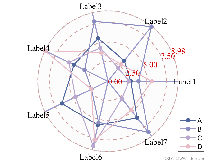
1.2.1 案例1:填充型
成图如下所示:

MATLAB实现代码如下:
clc
close all
clear
%% 导入数据
pathFigure= '.\Figures\' ;

%% Example 1
X = randi([2,8],[4,7])+rand([4,7]);

figure(1)
RC = radarChart(X ,'Type','Patch');
RC.RLim = [2,10];                         % 范围
RC.RTick = [2,8:1:10];                   % 刻度线
RC.PropName = {'Label1','Label2','Label3','Label4','Label5','Label6','Label7'};
RC.ClassName = {'A','B','C','D'};
RC = RC.draw();
RC.legend();                                 % 添加图例

colorList=[78 101 155;
          138 140 191;
          184 168 207;
          231 188 198;
          253 207 158;
          239 164 132;
          182 118 108]./255;
for n=1:RC.ClassNum
    RC.setPatchN(n,'FaceColor',colorList(n,:),'EdgeColor',colorList(n,:))
end

RC.setThetaTick('LineWidth',2,'Color',[.6,.6,.8]);          % theta轴颜色设置
RC.setRTick('LineWidth',1.5,'Color',[.8,.6,.6]);              % R轴颜色设置
RC.setPropLabel('FontSize',15,'FontName','Times New Roman','Color',[0,0,0])               % 属性标签
RC.setRLabel('FontSize',15,'FontName','Times New Roman','Color',[.8,0,0])                    % R刻度标签
% RC.setBkg('FaceColor',[0.8,0.8,0.8])                % 圆形背景颜色
% RC.setRLabel('Color','none')                           % 圆形背景颜色

str= strcat(pathFigure, "Figure1", '.tiff');
print(gcf, '-dtiff', '-r600', str);
1.2.2 案例2:线型
成图如下所示:
MATLAB实现代码如下:
clc
close all
clear
%% 导入数据
pathFigure= '.\Figures\' ;

%% Example 2
X = randi([2,8],[4,7])+rand([4,7]);

figure(2)
RC=radarChart(X ,'Type','Line');
RC.PropName = {'Label1','Label2','Label3','Label4','Label5','Label6','Label7'};
RC.ClassName = {'A','B','C','D'};
RC=RC.draw();
RC.legend();

colorList=[78 101 155;
          138 140 191;
          184 168 207;
          231 188 198;
          253 207 158;
          239 164 132;
          182 118 108]./255;
for n=1:RC.ClassNum
    RC.setPatchN(n,'Color',colorList(n,:),'MarkerFaceColor',colorList(n,:))
end

RC.setThetaTick('LineWidth',2,'Color',[.6,.6,.8]);          % theta轴颜色设置
RC.setRTick('LineWidth',1.5,'Color',[.8,.6,.6]);              % R轴颜色设置
RC.setPropLabel('FontSize',15,'FontName','Times New Roman','Color',[0,0,0])               % 属性标签
RC.setRLabel('FontSize',15,'FontName','Times New Roman','Color',[.8,0,0])                    % R刻度标签
% RC.setBkg('FaceColor',[0.8,0.8,0.8])                % 圆形背景颜色
% RC.setRLabel('Color','none')                           % 圆形背景颜色

str= strcat(pathFigure, "Figure2", '.tiff');
print(gcf, '-dtiff', '-r600', str);
2 方法二
函数来源为MATLAB帮助-spider_plot
2.1 调用函数
语法(Syntax):
spider_plot(P)

spider_plot(P, Name, Value, ...)

h = spider_plot(_)
输入变量:
- P:用于绘制蜘蛛图的数据点。行是数据组,列是数据点。如果没有指定轴标签和轴限制,则自动生成。[向量|矩阵]
输出变量:
- h:蜘蛛图的图柄。(图对象)
名称-值对参数(Name-Value Pair Arguments):
| 名称 | 说明 | 备注 |
|---|---|---|
| AxesLabels | 用于指定每个轴的标签 | [自动生成(默认)/单元格的字符串/ ‘none’] |
| AxesInterval | 用于更改显示在网页之间的间隔数 | [3(默认值)/ integer] |
| AxesPrecision | 用于更改轴上显示的值的精度级别 | [1(默认)/ integer / vector] |
| AxesDisplay | 用于更改显示轴文本的轴数。'None’或’one’可用于简化规范化数据的图形外观 | [‘none’(默认)/ “没有”/“一”/“数据”/“data-percent”] |
2.2 案例
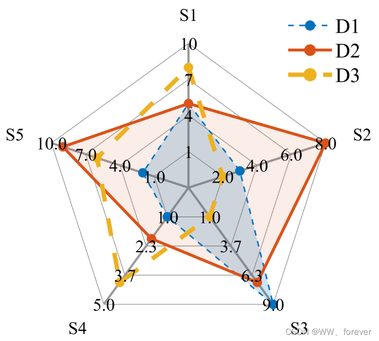
2.2.1 案例1:填充型
成图如下所示:

MATLAB实现代码如下:
clc
close all
clear
%% 导入数据
pathFigure= '.\Figures\' ;
%% Example 1
% Initialize data points
D1 = [5 3 9 1 2];
D2 = [5 8 7 2 9];
D3 = [8 2 1 4 6];
P = [D1; D2; D3];

% Spider plot
figure(1)
h = spider_plot(P,...
    'AxesLabels', {'S1', 'S2', 'S3', 'S4', 'S5'},...
    'FillOption', {'on', 'on', 'off'},...
    'FillTransparency', [0.2, 0.1, 0.1],...
    'AxesLimits', [1, 2, 1, 1, 1; 10, 8, 9, 5, 10],...             % [min axes limits; max axes limits]
    'AxesPrecision', [0, 1, 1, 1, 1],...
    'LineStyle', {'--', '-', '--'},...
    'LineWidth', [1, 2, 3],...
    'AxesFont', 'Times New Roman',...
    'LabelFont', 'Times New Roman',...
    'AxesFontSize', 12,...
    'LabelFontSize', 12,...
    'AxesLabelsEdge', 'none');


% Legend settings
hl = legend('D1', 'D2', 'D3', 'Location', 'northeast');
set(hl,'Box','off','FontSize',14,'Fontname', 'Times New Roman');

str= strcat(pathFigure, "Figure1", '.tiff');
print(gcf, '-dtiff', '-r600', str);
2.2.2 案例2:线型
成图如下所示:

MATLAB实现代码如下:
clc
close all
clear
%% 导入数据
pathFigure= '.\Figures\' ;
%% Example 2
% Initialize data points
D1 = [5 3 9 1 2 2 9 3 1 9 8 7 2 3 6];
D2 = [5 8 7 2 9 7 6 4 8 9 2 1 8 2 4];
D3 = [8 2 1 4 6 1 8 4 2 3 7 5 6 1 6];
P = [D1; D2; D3];

% Spider plot
spider_plot(P,...
    'AxesLimits', [0 0 0 0 0 0 0 0 0 0 0 0 0 0 0;...
    10 10 10 10 10 10 10 10 10 10 10 10 10 10 10],...
    'AxesInterval', 5,...
    'AxesDisplay', 'one',...
    'AxesPrecision', 0,...
    'AxesLabelsRotate', 'on',...
    'AxesLabelsOffset', 0.1,...
    'AxesRadial', 'off',...
     'AxesFont', 'Times New Roman',...
    'LabelFont', 'Times New Roman',...
    'AxesFontSize', 12,...
    'LabelFontSize', 12,...
    'AxesLabelsEdge', 'none');

% Legend settings
hl = legend('D1', 'D2', 'D3', 'Location', 'northeast');
set(hl,'Box','off','FontSize',14,'Fontname', 'Times New Roman');

str= strcat(pathFigure, "Figure2", '.tiff');
print(gcf, '-dtiff', '-r600', str);
2.2.3 案例3:绘制各月降水量
成图如下所示:

MATLAB绘图代码如下:
clc
close all
clear
%% 导入数据
pathFigure= '.\Figures\' ;

%% 开始绘图
figureUnits = 'centimeters';
figureWidth = 30;
figureHeight = 15;

figure(1)
set(gcf, 'Units', figureUnits, 'Position', [0 0 figureWidth figureHeight]);

pos1 = [0.05 0.1 0.3 0.8];
subplot('Position',pos1)
hold on;
box on;
spider_plot(PArea,...
    'AxesLabels', {'Jan.', 'Feb.', 'Mar.', 'Apr.', 'May','Jun.', 'Jul.', 'Aug.', 'Sep.', 'Oct.', 'Nov.', 'Dec.'},...
    'AxesLimits', [ones(1,12)*30 ; ones(1,12)*48 ],...
    'AxesInterval', 5,...
    'AxesDisplay', 'one',...
    'AxesPrecision', 0,...
    'AxesLabelsRotate', 'off',...
    'AxesLabelsOffset', 0.1,...
    'AxesRadial', 'on',...
     'AxesFont', 'Times New Roman',...
    'LabelFont', 'Times New Roman',...
    'AxesFontSize', 12,...
    'LabelFontSize', 12,...
    'AxesLabelsEdge', 'none');
text( 'string', "\fontname{Times New Roman}(a)\fontname{宋体}各月降水量\fontname{Times New Roman}/mm", 'Units','normalized','position',[0.02,1.05],  'FontSize',14,'FontWeight','Bold');


pos2 = [0.43 0.15 0.56 0.7];
subplot('Position',pos2)
hold on;
box on;
h(1) = plot(PAreaYear,'-o','LineWidth',1.5,'color',[77,133,189]/255,'MarkerEdgeColor',[77,133,189]/255,'MarkerFaceColor',[77,133,189]/255,'Markersize',5);
h(2) = plot(1:nYear, PAreaYearfit ,'--','color',[40 120 181]/255,'LineWidth',1);
xlabel("\fontname{宋体}\fontsize{15}年份",'FontName','宋体','FontSize',12);                          % 后续调整坐标标题
ylabel("\fontname{宋体}\fontsize{15}降水\fontname{Times New Roman}\fontsize{15}/mm",'FontSize',12);                          % 后续调整坐标标题
text( 'string', "\fontname{Times New Roman}(b)\fontname{宋体}年降水", 'Units','normalized','position',[0.02,1.05],  'FontSize',14,'FontWeight','Bold');
set(gca,'xlim',[0  nYear+1],'xtick',[1:5:nYear+1],'xticklabel', [yearStart :5:yearEnd] ,'FontSize',12,'FontName','Times New Roman','XMinorTick','on');
text( nYear/2-3.5,550 ,"y= "+roundn( P(1,1),-4) +"x+"+roundn( P(1,2),-4) , 'color','k', 'FontSize',12,'FontName','Times New Roman' );
text( nYear/2-3.5,535 ,"R^2= "+ roundn(R,-4) , 'color','k', 'FontSize',12,'FontName','Times New Roman' );
ax = gca;
ax.XAxis.MinorTickValues = 1:1:nYear+1;
set(gca,'ylim',[300 650],'ytick',[300:50:620],'yticklabel',[300:50:620],'FontSize',12,'FontName','Times New Roman');
hl = legend(h([1 2]), "年降水","线性(年降水)" );
set(hl,'Box','off','location','NorthEast','NumColumns',2,'FontSize',12,'FontName','宋体');
set(gca,'Layer','top');

str= strcat(pathFigure, "Figure1", '.tiff');
print(gcf, '-dtiff', '-r600', str);
参考
1.MATLAB | 如何使用MATLAB绘制雷达图(蜘蛛图)
2.MATLAB帮助-spider_plot

旨在为数千万中国开发者提供一个无缝且高效的云端环境,以支持学习、使用和贡献开源项目。
更多推荐


 14
14 0
0- 0


 已为社区贡献23条内容

所有评论(0)