Hans Moravec，占用栅格地图的发明人。

 

Obstacle Avoidance and Navigation in the Real World by a Seeing Robot Rover

 

Hans Moravec
March 1980
Computer Science Department
Stanford University
(Ph.D. thesis)

Preface

The Stanford AI lab cart is a card-table sized mobile robot controlled remotely through a radio link, and equipped with a TV camera and transmitter. A computer has been programmed to drive the cart through cluttered indoor and outdoor spaces, gaining its knowledge about the world entirely from images broadcast by the onboard TV system.

The cart deduces the three dimensional location of objects around it, and its own motion among them, by noting their apparent relative shifts in successive images obtained from the moving TV camera. It maintains a model of the location of the ground, and registers objects it has seen as potential obstacles if they are sufficiently above the surface, but not too high. It plans a path to a user-specified destination which avoids these obstructions. This plan is changed as the moving cart perceives new obstacles on its journey.

The system is moderately reliable, but very slow. The cart moves about one meter every ten to fifteen minutes, in lurches. After rolling a meter, it stops, takes some pictures and thinks about them for a long time. Then it plans a new path, and executes a little of it, and pauses again.

The program has successfully driven the cart through several 20 meter indoor courses (each taking about five hours) complex enough to necessitate three or four avoiding swerves. A less sucessful outdoor run, in which the cart swerved around two obstacles but collided with a third, was also done. Harsh lighting (very bright surfaces next to very dark shadows) resulting in poor pictures, and movement of shadows during the cart's creeping progress, were major reasons for the poorer outdoor performance. These obstacle runs have been filmed (minus the very dull pauses).

Hans Moravec
March 2, 1980

 

Table of Contents

Chapter 1:   Introduction
Chapter 2:   History
Chapter 3:   Overview
Chapter 4:   Calibration
Chapter 5:   Interest Operator
Chapter 6:   Correlation
Chapter 7:   Stereo
Chapter 8:   Path Planning
Chapter 9:   Evaluation
Chapter 10:   Spinoffs
Chapter 11:   Future Carts
Chapter 12:   Connections

Appendix 1:   Introduction
Appendix 2:   History
Appendix 3:   Overview
Appendix 6:   Correlation
Appendix 7:   Stereo
Appendix 8:   Path Planning
Appendix 10:   Spinoffs
Appendix 12:   Connections

 

Acknowledgements

My nine year stay at the Stanford AI lab has been pleasant, but long enough to tax my memory. I hope not too many people have been forgotten.

Rod Brooks helped with most aspects of this work during the last two years and especially during the grueling final weeks before the lab move in 1979. Without his help my PhD-hood might have taken ten years.

Vic Scheinman has been a patron saint of the cart project since well before my involvement. Over the years he has provided untold many motor and sensor assemblies, and general mechanical expertise whenever requested. His latest contribution was the camera slider assembly which is the backbone of the cart's vision.

Don Gennery provided essential statistical geometry routines, and many useful discussions.

Mike Farmwald wrote several key routines in the display and vision software packages used by the obstacle avoider, and helped construct some of the physical environment which made cart operations pleasant.

Jeff Rubin pleasantly helped with the electronic design of the radio control link and other major components.

Marvin Horton provided support and an array of camera equiment, including an impressive home built ten meter hydraulic movie crane for the filming of the final cart runs.

Others who have helped recently are Harlyn Baker, Peter Blicher, Dick Gabriel, Bill Gosper, Elaine Kant, Mark LeBrun, Robert Maas, Allan Miller, Lynne Toribara and Polle Zellweger.

My debts in the farther past are many, and my recollection is sporadic. I remember particularly the difficult time reconstructing the cart's TV transmitter. Bruce Bullock, Tom Gafford, Ed McGuire and Lynn Quam made it somewhat less traumatic.

Delving even farther, I wish to thank Bruce Baumgart for radiating a pleasantly (and constructively) wild eyed attitude about this line of work, and Rod Schmidt, whom I have never met, for building the hardware that made my first five years of cart work possible.

In addition I owe very much to the unrestrictive atmosphere created at the lab mainly by John McCarthy and Les Earnest, and maintained by Tom Binford, and also to the excellent system support provided to me (over the years) by Marty Frost, Ralph Gorin, Ted Panofsky and Robert Poor.

Hans Moravec, 1980

Chapter 1: Introduction

This is a report about a modest attempt at endowing a mild mannered machine with a few of the attributes of higher animals.

An electric vehicle, called the cart, remote controlled by a computer, and equipped with a TV camera through which the computer can see, has been programmed to run undemanding but realistic obstacle courses.

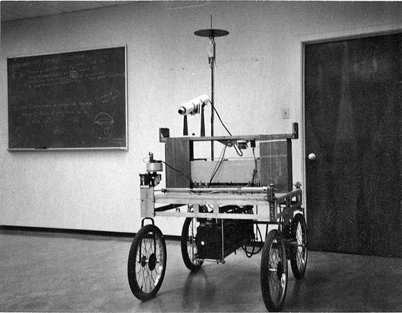
Figure 1.1: The cart, like a card table, but taller

The methods used are minimal and crude, and the design criteria were simplicity and performance. The work is seen as an evolutionary step on the road to intellectual development in machines. Similar humble experiments in early vertebrates eventually resulted in human beings.

Figure 1.2: SRI's Shakey and JPL's Robotics Research Vehicle

The hardware is also minimal. The television camera is the cart's only sense organ. The picture perceived can be converted to an array of numbers in the computer of about 256 rows and 256 columns, with each number representing up to 64 shades of gray. The cart can drive forwards and back, steer its front wheels and move its camera from side to side. The computer controls these functions by turning motors on and off for specific lengths of time.

Better (at least more expensive) hardware has been and is being used in similar work elsewhere. SRI's Shakey moved around in a contrived world of giant blocks and clean walls. JPL is trying to develop a semi-autonomous rover for the exploration of Mars and other far away places (the project is currently mothballed awaiting resumption of funding). Both SRI's and JPL's robots use laser rangefinders to determine the distance of nearby objects in a fairly direct manner. My system, using less hardware and more computation, extracts the distance information from a series of still pictures of the world from different points of view, by noting the relative displacement of objects from one picture to the next.

 

Applications

 

A Mars rover is the most likely near term use for robot vehicle techniques. The half hour radio delay between Earth and Mars makes direct remote control an unsatisfactory way of guiding an exploring device. Automatic aids, however limited, would greatly extend its capabilities. I see my methods as complementary to approaches based on rangefinders. A robot explorer will have a camera in addition to whatever other sensors it carries. Visual obstacle avoidance can be used to enhance the reliability of other methods, and to provide a backup for them.

Robot submersibles are almost as exotic as Mars rovers, and may represent another not so distant application of related methods. Remote control of submersibles is difficult because water attenuates conventional forms of long distance communication. Semi-autonomous minisubs could be useful for some kinds of exploration and may finally make seabed mining practical.

In the longer run the fruits of this kind of work can be expected to find less exotic uses. Range finder approaches to locating obstacles are simpler because they directly provide the small amount of information needed for undemanding tasks. As the quantity of information to be extracted increases the amount of processing, regardless of the exact nature of the sensor, will also increase.

What a smart robot thinks about the world shouldn't be affected too much by exactly what it sees with. Low level processing differences will be mostly gone at intermediate and high levels. Present cameras offer a more detailed description of the world than contemporary rangefinders and camera based techniques probably have more potential for higher visual functions.

The mundane applications are more demanding than the rover task. A machine that navigates in the crowded everyday world, whether a robot servant or an automatic car, must efficiently recognize many of the things it encounters to be safe and effective. This will require methods and processing power beyond those now existing. The additional need for low cost guarantees they will be a while in coming. On the other hand work similar to mine will eventually make them feasible.

 

Chapter 2: History

This work was shaped to a great extent by its physical circumstances; the nature and limitations of the cart vehicle itself, and the resources that could be brought to bear on it. The cart has always been the poor relation of the Stanford Hand-Eye project, and has suffered from lack of many things, not the least of which was sufficient commitment and respect by any principal investigator.

The cart was built in the early 1960's by a group in the Stanford Mechanical Engineering Department under a NASA contract, to investigate potential solutions for the problems of remote controlling a lunar rover from Earth. The image from an onboard TV camera was broadcast to a human operator who manipulated a steering control. The control signals were delayed for two and a half seconds by a tape loop, then broadcast to the cart, simulating the Earth/Moon round trip delay.

The AI lab, then in its enthusiastic spit and baling wire infancy, acquired the cart gratis from ME after they were done, minus its video and remote control electronics. Rod Schmidt, an EE graduate student and radio amateur was induced to work on restoring the vehicle, and driving it under computer control. He spent over two years, but little money, single-handedly building a radio control link based on a model airplane controller, and a UHF TV link. The control link was relatively straightforward, the video receiver was a modified TV set, but the UHF TV transmitter took 18 laborious months of tweaking tiny capacitors and half centimeter turns of wire. The resulting robot was ugly, reflecting its rushed assembly, and marginally functional (the airplane proportional controller was very inaccurate). Like an old car, it needed (and needs) constant repair and replacement of parts, major and minor, that break.

Schmidt then wrote a program for the PDP-6 which drove the cart in real time (but with its motors set to run very slowly) along a wide white line. It worked occasionally. Following a white line with a raised TV camera and a computer turns out to be much more difficult than following a line at close range with a photocell tracker. The camera scene is full of high contrast extraneous detail, and the lighting conditions are unreliable. This simple program taxed the processing power of the PDP-6. It also clearly demonstrated the need for more accurate and reliable hardware if more ambitious navigation problems were to be tackled. Schmidt wrote up the results and finished his degree.

Bruce Baumgart picked up the cart banner, and announced an ambitious approach that would involve modelling the world in great detail, and by which the cart could deduce its position by comparing the image it saw through its camera with images produced from its model by a 3D drawing program. He succeeded reasonably well with the graphics end of the problem.

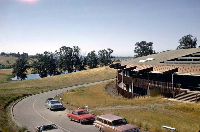
Figure 2.1: The old AI lab and some of the surrounding terrain, about 1968

The real world part was a dismal failure. He began with a rebuild of the cart control electronics, replacing the very inaccurate analog link with a supposedly more repeatable digital one. He worked as single-handedly as did Schmidt, but without the benefit of prior experience with hardware construction. The end result was a control link that, because of a combination of design flaws and undetected bugs, was virtually unusable. One time out of three the cart moved in a direction opposite to which it had been commanded, left for right or forwards for backwards.

During this period a number of incoming students were assigned to the “cart project”. Each correctly perceived the situation within a year, and went on to something else. The cart's reputation as a serious piece of research apparatus, never too high, sank to new depths.

I came to the AI lab, enthusiastic and naive, with the specific intention of working with the cart. I'd built a series of small robots, beginning in elementary school, and the cart, of whose existence, but not exact condition, I'd learned, seemed like the logical next step. Conditions at the lab were liberal enough that my choice was not met with termination of financial support, but this largesse did not easily extend to equipment purchases.

Lynn Quam, who had done considerable work with stereo mapping from pictures from the Mariners 6 and 7 Mars missions, expressed an interest in the cart around this time, for its clear research value for Mars rovers. We agreed to split up the problem (the exact goals for the collaboration were never completely clear; mainly they were to get the cart to do as much as possible). He would do the vision, and I would get the control hardware working adequately and write motor subroutines which could translate commands like move a meter forward and a half to the right into appropriate steering and drive signals.

I debugged, then re-designed and rebuilt the control link to work reliably, and wrote a routine that incorporated a simulation of the cart, to drive it (this subroutine was resurrected in the final months of the obstacle avoider effort, and is described in chapter 8). I was very elated by my quick success, and spent considerable time taking the cart on joy rides. I would open the big machine room doors near the cart's parking place, and turn on the cart. Then I would rush to my office, tune in the cart video signal on a monitor, start a remote control program, and, in armchair and air conditioned comfort, drive the cart out the doors. I would steer it along the outer deck of the lab to one of three ramps on different sides of the building. I then drove it down the narrow ramp (they were built for deliveries), and out into the driveway or onto the grass, to see (on my screen) what there was to see. Later I would drive it back the same way, then get up to close the doors and power it down. With increasing experience, I became increasingly cocky. During the 1973 IJCAI, held at Stanford, I repeatedly drove it up and down the ramps, and elsewhere, for the amusement of the crowds visiting the AI lab during an IJCAI sponsored winetasting.

Shortly after the IJCAI my luck ran out. Preparing to drive it down the front ramp for a demonstration, I misjudged the position of the right edge by a few centimeters. The cart's right wheels missed the ramp, and the picture on my screen slowly rotated 90°, then turned into noise. Outside, the cart was lying on its side, with acid from its batteries spilling into the electronics. Sigh.

The sealed TV camera was not damaged. The control link took less than a month to resurrect. Schmidt's video transmitter was another matter. I spent a total of nine frustrating months first trying, unsuccessfully, to repair it, then building (and repeatedly rebuilding) a new one from the old parts using a cleaner design found in a ham magazine and a newly announced UHF amplifier module from RCA. The new one almost worked, though its tuning was touchy. The major problem was a distortion in the modulation. The RCA module was designed for FM, and did a poor job on the AM video signal. Although TV sets found the broadcast tolerable, our video digitizer was too finicky.

During these nine difficult months I wrote to potential manufacturers of such transmitters, and also inquired about borrowing the video link used by Shakey, which had been retired by SRI. SRI, after due deliberation, turned me down. Small video transmitters are not off the shelf items; the best commercial offer I got was for a two watt transmitter costing $4000.

Four kilobucks was an order of magnitude more money than had ever been put into cart hardware by the AI lab, though it was was considerably less than had been spent on salary in Schmidt's 18 months and my 9 months of transmitter hacking. I begged for it and got an agreement from John McCarthy that I could buy a transmitter, using ARPA money, after demonstrating a capability to do vision.

During the next month I wrote a program that picked a number of features in one picture (the “interest operator” of Chapter 5 was invented here) of a motion stereo pair, and found them in the other image with a simple correlator, did a crude distance calculation, and generated a fancy display. Apparently this was satisfactory; the transmitter was ordered.

By this time Quam had gone on to other things. With the cart once again functional, I wrote a program that drove it down the road in a straight line by servoing on points it found on the distant horizon with the interest operator and tracked with the correlator. Like the current obstacle avoider, it did not run in real time, but in lurches. That task was much easier, and even on the KA-10, our main processor at the time, each lurch took at most 15 seconds of real time. The distance travelled per lurch was variable; as small as a quarter meter when the program detected significant variations from its desired straight path, repeatedly doubling up to many meters when everything seemed to be working. The program also observed the cart's response to commands, and updated a response model which it used to guide future commands. The program was reliable and fun to watch, except that the remote control link occasionally failed badly. The cause appeared to be interference from passing CBers. The citizens band boom had started, and our 100 milliwatt control link, which operated in the CB band, was not up to the competition.

I replaced the model airplane transmitter and receiver by standard (but modified) CB transceivers, increasing the broadcast power to 5 watts. To test this and a few other improvements in the hardware, I wrote an updated version of the horizon tracker which incorporated a new idea, the faster and more powerful “binary search” correlator of Chapter 6. This was successful, and I was ready for bigger game.

Obstacle avoidance could be accomplished using many of the techniques in the horizon tracker. A dense cloud of features on objects in the world could be tracked as the cart rolled forward, and a 3D model of their position and the cart's motion through them could be deduced from their relative motion in the image. Don Gennery had already written a camera solving subroutine, used by Quam and Hannah, which was capable of such a calculation.

I wrote a program which drove the cart, tracking features near and far, and feeding them to Gennery's subroutine. The results were disappointing. Even after substantial effort, aggravated by having only a very poor a priori model of cart motion, enough of the inevitable correlation errors escaped detection to make the camera solver converge to the wrong answer about 10 to 20% of the time. This error rate was too high for a vehicle that would need to navigate through at least tens of such steps. Around this time I happened to catch some small lizards, that I kept for a while in a terrarium. Watching them, I observed an interesting behavior.

The lizards caught flies by pouncing on them. Since flies are fast, this requires speed and 3D precision. Each lizard had eyes on opposite sides of its head; the visual fields could not overlap significantly, ruling out stereo vision. But before a pounce, a lizard would fix an eye on its victim, and sway its head slowly from side to side. This seemed a sensible way to range.

My obstacle avoiding task was defeating the motion stereo approach, and the lizard's solution seemed promising. I built a stepping motor mechanism that could slide the cart's camera from side to side in precise increments. The highly redundant information available from this apparatus broke the back of the problem, and made the obstacle avoider that is the subject of this thesis possible.

Chapter 3: Overview

A typical run of the avoider system begins with a calibration of the cart's camera. The cart is parked in a standard position in front of a wall of spots. A calibration program (described in Chapter 4) notes the disparity in position of the spots in the image seen by the camera with their position predicted from an idealized model of the situation. It calculates a distortion correction polynomial which relates these positions, and which is used in subsequent ranging calculations.

Figure 3.1: The cart in its calibration pose

The cart is then manually driven to its obstacle course. Typically this is either in the large room in which it lives, or a stretch of the driveway which encircles the AI lab. Chairs, boxes, cardboard constructions and assorted debris serve as obstacles in the room. Outdoors the course contains curbing, trees, parked cars and signposts as well.

Figure 3.2: The cart indoors

Figure 3.3: The cart outdoors

The obstacle avoiding program is started. It begins by asking for the cart's destination, relative to its current position and heading. After being told, say, 50 meters forward and 20 to the right, it begins its maneuvers.

It activates a mechanism which moves the TV camera, and digitizes about nine pictures as the camera slides (in precise steps) from one side to the other along a 50 cm track.

Figure 3.4: A closeup of the slider mechanism

 

A subroutine called the interest operator (described in Chapter 5) is applied to the one of these pictures. It picks out 30 or so particularly distinctive regions (features) in this picture. Another routine called the correlator (Chapter 6) looks for these same regions in the other frames. A program called the camera solver (Chapter 7) determines the three dimensional position of the features with respect to the cart from their apparent movement image to image.

The navigator (Chapter 8) plans a path to the destination which avoids all the perceived features by a large safety margin. The program then sends steering and drive commands to the cart to move it about a meter along the planned path. The cart's response to such commands is not very precise.

After the step forward the camera is operated as before, and nine new images are acquired. The control program uses a version of the correlator to find as many of the features from the previous location as possible in the new pictures, and applies the camera solver. The program then deduces the cart's actual motion during the step from the apparent three dimensional shift of these features.

The motion of the cart as a whole is larger and less constrained than the precise slide of the camera. The images between steps forward can vary greatly, and the correlator is usually unable to find many of the features it wants. The interest operator/correlator/camera solver combination is used to find new features to replace lost ones.

The three dimensional location of any new features found is added to the program's model of the world. The navigator is invoked to generate a new path that avoids all known features, and the cart is commanded to take another step forward.

This continues until the cart arrives at its destination or until some disaster terminates the program.

Appendix 3 documents the evolution of the cart's internal world model in response to the scenery during a sample run.

An Objection

A method as simple as this is unlikely to handle every situation well. The most obvious problem is the apparently random choice of features tracked. If the interest operator happens to avoid choosing any points on a given obstruction, the program will never notice it, and might plan a path right through it.

The interest operator was designed to minimize this danger. It chooses a relatively uniform scattering of points over the image, locally picking those with most contrast. Effectively it samples the picture at low resolution, indicating the most promising regions in each sample area.

Objects lying in the path of the vehicle occupy ever larger areas of the camera image as the cart rolls forward. The interest operator is applied repeatedly, and the probability that it will choose a feature or two on the obstacle increases correspondingly. Typical obstructions are generally detected before its too late. Very small or very smooth objects are sometimes overlooked.

Chapter 4: Calibration

Figure 4.1: The cart in its calibration posture before the calibration pattern. A program automatically locates the cross and the spots, and deduces the camera's focal length and distortion.

The cart camera, like most vidicons, has peculiar geometric properties. Its precision has been enhanced by an automatic focal length and distortion determining program.

The cart is parked a precise distance in front of a wall of many spots and one cross (Figure 4.1). The program digitizes an image of the spot array, locates the spots and the cross, and constructs a a two dimensional polynomial that relates the position of the spots in the image to their position in an ideal unity focal length camera, and another polynomial that converts points from the ideal camera to points in the image. These polynomials are used to correct the positions of perceived objects in later scenes.

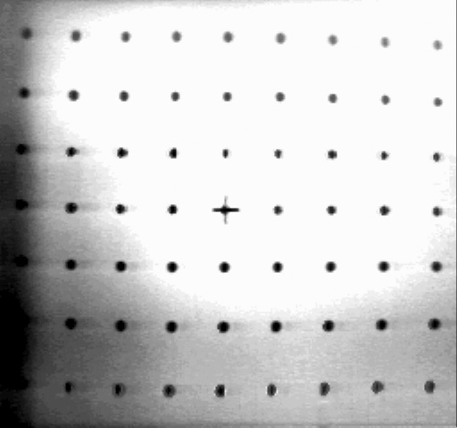
Figure 4.2: The spot array, as digitized by the cart camera

The program tolerates a wide range of spot parameters (about 3 to 12 spots across), arbitrary image rotation, and is very robust. After being intensely fiddled with to work successfully on an initial set of 20 widely varying images, it has worked without error on 50 successive images. The test pattern for the cart is a 3 meter square painted on a wall, with 5 cm spots at 30 cm intervals. The program has also been used successfully with a small array (22 x 28 cm) to calibrate cameras other than the cart's \ref(W1).

 

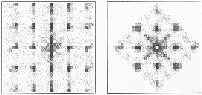
Figure 4.3: Power spectrum of Figure 4.2, and folded transform

Figure 4.4: Results of the calibration program. The distortion polynomial it produced has been used to map an undistorted grid of ideal spot positions into the calculated real world ones. The result is superimposed on the original digitized spot image, making any discrepancies obvious.

 

Figure 4.5: Another instance of the distortion corrector at work; a longer focal length lens

 

Figure 4.6: Yet another example; a rotation

 

Figure 4.7: And yet another example

The algorithm reads in an image of such an array, and begins by determining its approximate spacing and orientation. It trims the picture to make it square, reduces it by averaging to 64 by 64, calculates the Fourier transform of the reduced image and takes its power spectrum, arriving at a 2D transform symmetric about the origin, and having strong peaks at frequencies corresponding to the horizontal and vertical and half-diagonal spacings, with weaker peaks at the harmonics. It multiplies each point $[i,j]$ in this transform by point $[-j,i]$ and points $[j-i,j+i]$ and $[i+j,j-i]$, effectively folding the primary peaks onto one another. The strongest peak in the 90° wedge around the $Y$ axis gives the spacing and orientation information needed by the next part of the process.

The directional variance interest operator described later (Chapter 5) is applied to roughly locate a spot near the center of the image. A special operator examines a window surrounding this position, generates a histogram of intensity values within the window, decides a threshold for separating the black spot from the white background, and calculates the centroid and first and second moment of the spot. This operator is again applied at a displacement from the first centroid indicated by the orientation and spacing of the grid, and so on, the region of found spots growing outward from the seed.

A binary template for the expected appearance of the cross in the middle of the array is constructed from the orientation/spacing determined determined by the Fourier transform step. The area around each of the found spots is thresholded on the basis of the expected cross area, and the resulting two valued pattern is convolved with the cross template. The closest match in the central portion of the picture is declared to be the origin.

Two least-squares polynomials (one for $X$ and one for $Y$) of third (or sometimes fourth) degree in two variables, relating the actual positions of the spots to the ideal positions in a unity focal length camera, are then generated and written into a file.

The polynomials are used in the obstacle avoider to correct for camera roll, tilt, focal length and long term variations in the vidicon geometry.

Chapter 5: Interest Operator

The cart vision code deals with very simple primitive entities, localized regions called features. A feature is conceptually a point in the three dimensional world, but it is found by examining localities larger than points in pictures. A feature is good if it can be located unambiguously in different views of a scene. A uniformly colored region or a simple edge does not make for good features because its parts are indistinguishable. Regions, such as corners, with high contrast in orthogonal directions are best.

New features in images are picked by a subroutine called the interest operator, an example of whose operation is displayed in Figure 5-1. It tries to select a relatively uniform scattering, to maximize the probability that a few features will be picked on every visible object, and to choose areas that can be easily found in other images. Both goals are achieved by returning regions that are local maxima of a directional variance measure. Featureless areas and simple edges, which have no variance in the direction of the edge, are thus avoided.

Figure 5.1: A cart's eye view from the starting position of an obstacle run, and features picked out by the interest operator. They are labelled in order of decreasing interest measure.

Figure 5.2: A typical interest operator window, and the four sums calculated over it ($P_{I,J}$ are the pixel bightnesses). The interest measure of the window is the minimum of the four sums.

Figure 5.3: The twenty five overlapping windows considered in a local maximum decision. The smallest cells in the diagram are individual pixels. The four by four array of these in the center of the image is the window being considered as a local maximum. In order for it to be chosen as a feature to track, its interest measure must equal or exceed that of each of the other outlined four by four areas.

Directional variance is measured over small square windows. Sums of squares of differences of pixels adjacent in each of four directions (horizontal, vertical and two diagonals) over each window are calculated, and the window's interest measure is the minimum of these four sums.

Features are chosen where the interest measure has local maxima. The feature is conceptually the point at the center of the window with this locally maximal value.

This measure is evaluated on windows spaced half a window width apart over the entire image. A window is declared to contain an interesting feature if its variance measure is a local maximum, that is, if it has the largest value of the twenty five windows which overlap or contact it.

The variance measure depends on adjacent pixel differences and responds to high frequency noise in the image. The effects of noise are alleviated and the processing time is shortened by applying the operator to a reduced image. In the current program original images are 240 lines high by 256 pixels wide. The interest operator is applied to the 120 by 128 version, on windows 3 pixels square.

Figure 5.4: Another obstacle run interest operator application

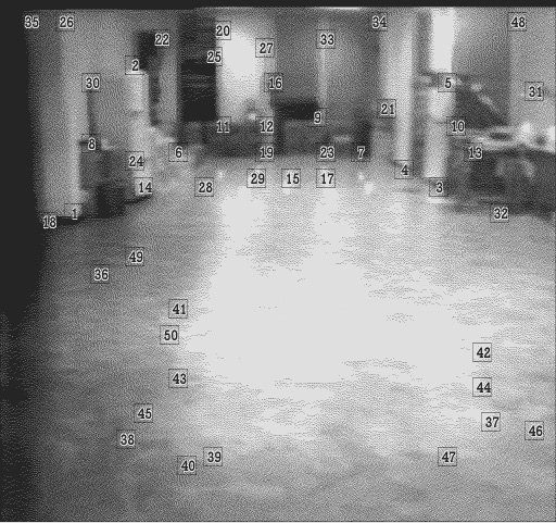
Figure 5.5: More interest operating

The local maxima found are stored in an array, sorted in order of decreasing variance.

The entire process on a typical 260 by 240 image, using 6 by 6 windows takes about 75 milliseconds on the KL-10. The variance computation and local maximum test are coded in FAIL (our assembler) \ref(WG1), the maxima sorting and top level are in SAIL (an Algol-like language) \ref(R1).

Once a feature is chosen, its appearance is recorded as series of excerpts from the reduced image sequence. A window (6 by 6 in the current implementation) is excised around the feature's location from each of the variously reduced pictures. Only a tiny fraction of the area of the original (unreduced) image is extracted. Four times as much of the x2 reduced image is stored, sixteen times as much of the x4 reduction, and so on until at some level we have the whole image. The final result is a series of 6 by 6 pictures, beginning with a very blurry rendition of the whole picture, gradually zooming in linear expansions of two to a sharp closeup of the feature. Of course, it records the appearance correctly from only one point of view.

Weaknesses

The interest operator has some fundamental limitations. The basic measure was chosen to reject simple edges and uniform areas. Edges are not suitable features for the correlator because the different parts of an edge are indistinguishable.

The measure is able to unambiguously reject edges only if they are oriented along the four directions of summation. Edges whose angle is an odd multiple of 22.5° give non-zero values for all four sums, and are sometimes incorrectly chosen as interesting.

The operator especially favors intersecting edges. These are sometimes corners or cracks in objects, and are very good. Sometimes they are caused by a distant object peering over the edge of a nearby one and then they are very bad. Such spurious intersections don't have a definite distance, and must be rejected during camera solving. In general they reduce the reliability of the system.

Desirable Improvements

The operator has a fundamental and central role in the obstacle avoider, and is worth improving. Edge rejection at odd angles should be increased, maybe by generating sums in the 22.5° directions.

Rejecting near/far object intersections more reliably than the current implementation does is possible. An operator that recognized that the variance in a window was restricted to one side of an edge in that window would be a good start. Really good solutions to this problem are probably computationally much more expensive than my measure.

Chapter 6: Correlation

Deducing the 3D location of features from their projections in 2D images requires that we know their position in two or more such images.

The correlator is a subroutine that, given a description of a feature as produced by the interest operator from one image, finds the best match in a different, but similar, image. Its search area can be the entire new picture, or a rectangular sub-window.

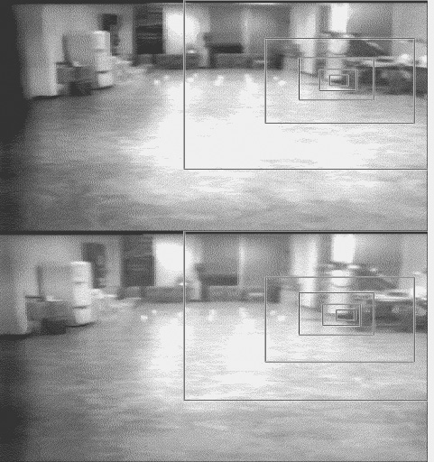
Figure 6.1: Areas matched in a binary search correlation. Picture at top contains originally chosen feature. The outlined areas in it are the prototypes which are searched for in the bottom picture. The largest rectangle is matched first, and the area of best match in the second picture becomes the search area for the next smaller rectangle. The larger the rectangle, the lower the resolution of the pictures in which the matching is done.

 

Figure 6.2: The “conventional” representation of a feature used in documents such as this one, and a more realistic version which graphically demonstrates the reduced resolution of the larger windows. The bottom picture was reconstructed entirely from the window sequence used with a binary search correlation. The coarse outer windows were interpolated to reduce quantization artifacts.

The search uses a coarse to fine strategy, illustrated in Figure 6-1, that begins in reduced versions of the pictures. Typically the first step takes place at the $\times 16$ (linear) reduction level. The $6 \times 6$ window at that level in the feature description, that covers about one seventh of the total area of the original picture, is convolved with the search area in the correspondingly reduced version of the second picture. The $6 \times 6$ description patch is moved pixel by pixel over the approximately $15$ by $16$ destination picture, and a correlation coefficient is calculated for each trial position.

The position with the best match is recorded. The $6 \times 6$ area it occupies in the second picture is mapped to the $\times 8$ reduction level, where the corresponding region is $12$ pixels by $12$. The $6 \times 6$ window in the $\times 8$ reduced level of the feature description is then convolved with this $12$ by $12$ area, and the position of best match is recorded and used as a search area for the $\times 4$ level.

The process continues, matching smaller and smaller, but more and more detailed windows until a $6 \times 6$ area is selected in the unreduced picture.

The work at each level is about the same, finding a $6 \times 6$ window in a $12$ by $12$ search area. It involves 49 summations of 36 quantities. In our example there were 5 such levels. The correlation measure used is ${2\sum ab}/({\sum a^2}+{\sum b^2})$, where $a$ and $b$ are the values of pixels in the two windows being compared, with the mean of windows subtracted out, and the sums are taken over the $36$ elements of a $6 \times 6$ window. The measure has limited tolerance to contrast differences.

The window sizes and other parameters are sometimes different from the ones used in this example.

In general, the program thus locates a huge general area around the feature in a very coarse version of the images, and successively refines the position, finding smaller and smaller areas in finer and finer representations. For windows of size $n$, the work at each level is approximately that of finding an $n$ by $n$ window in a $2n$ by $2n$ area, and there are $\log_2(w/n)$ levels, where $w$ is the smaller dimension of the search rectangle, in unreduced picture pixels.

This approach has many advantages over a simple pass of of a correlation coefficient computation over the search window. The most obvious is speed. A scan of an $8 \times 8$ window over a $256$ by $256$ picture would require $249 \times 249 \times 8 \times 8$ comparisons of individual pixels. The binary method needs only about $5 \times 81 \times 8 \times 8$, about $150$ times fewer. The advantage is lower for smaller search areas. Perhaps more important is the fact that the simple method exhibits a serious jigsaw puzzle effect. The $8 \times 8$ patch is matched without any reference to context, and a match is often found in totally unrelated parts of the picture. The binary search technique uses the general context to guide the high resolution comparisons. This makes possible yet another speedup, because smaller windows can be used. Window sizes as small as $2 \times 2$ work reasonably well. The searches at very coarse levels rarely return mismatches, possibly because noise is averaged out in the reduction process, causing comparisons to be more stable. Reduced images are also more tolerant of geometric distortions.

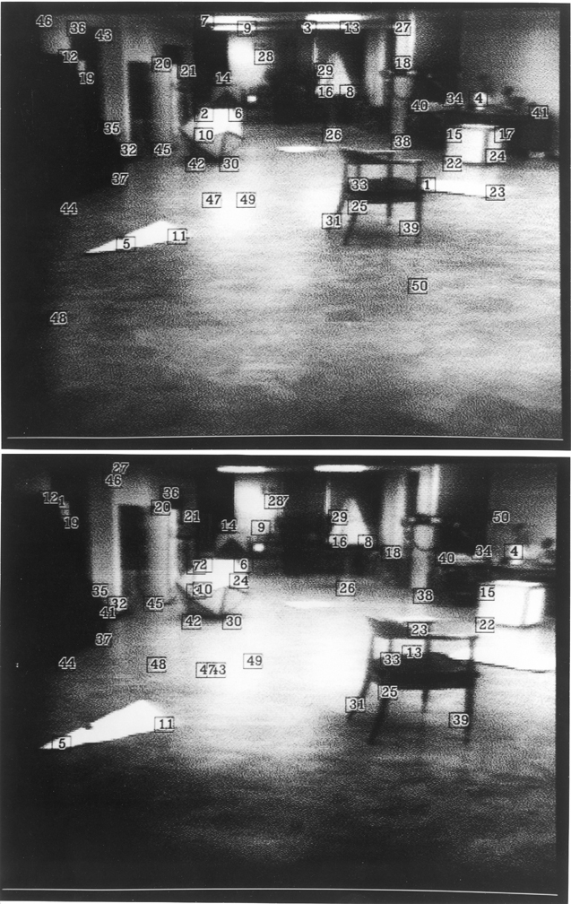
Figure 6.3: Example of the correlator's performance on a difficult example. The interest operator has chosen features in the upper image, and the correlator has attempted to find corresponding regions in the lower one. The cart moved about one and a half meters forward between the images. Some mistakes are evident. The correlator had no a-priori knowledge about the relationship of the two images and the entire second image was searched for each feature.

Figure 6.4: An outdoor application of the binary search correlator

The current routine uses a measure for the measure for the cross correlation which I call pseudo normalized, given by the formula $${2 \sum{ab} \over \sum{a^2} + \sum{b^2}}$$ that has limited contrast sensitivity, avoids the degeneracies of normalized correlation on informationless windows, and is slightly cheaper to compute. A description of its derivation may be found in Appendix 6.

Timing

The formula above is expressed in terms of $A$ and $B$ with the means subtracted out. It can be translated into an expression involving $\sum{A}$, $\sum{A^2}$, $\sum{B}$, $\sum{B^2}$ and $\sum{(A-B)^2}$. By evaluating the terms involving only $A$, the source window, outside of the main correlation loop, the work in the inner loop can be reduced to evaluating $\sum{B}$, $\sum{B^2}$ and $\sum{(A-B)^2}$. This is done in three PDP-10 machine instructions per point by using a table in which entry $i$ contains both $i$ and $i^2$ in subfields, and by generating in-line code representing the source window, three instructions per pixel, eliminating the need for inner loop end tests and enabling the $A-B$ computation to be done during indexing.

Each pixel comparison takes about one microsecond. The time required to locate an $8 \times 8$ window in a $16$ by $16$ search area is about $10$ milliseconds. A single feature requires $5$ such searches, for a total per feature time of $50$ ms.

One of the three instructions could be eliminated if $\sum{B}$ and $\sum{B^2}$ were precomputed for every position in the picture. This can be done incrementally, involving examination of each pixel only twice, and would result in an overall speedup if many features are to be searched for in the same general area.

The correlator has approximately a 10% error rate on features selected by the interest operator in our sample pictures. Typical image pairs are generally taken about two feet apart with a $60$° field of view camera.

Chapter 7: Stereo

Slider Stereo

At each pause on its computer controlled itinerary the cart slides its camera from left to right on the 52 cm track, taking 9 pictures at precise 6.5 cm intervals.

Points are chosen in the fifth (middle) of these 9 images, either by the correlator to match features from previous positions, or by the interest operator.

 

Figure 7.1: A typical ranging. The nine pictures are from a slider scan. The interest operator chose the marked feature in the central image, and the correlator found it in the other eight. The small curves at bottom are distance measurements of the feature made from pairs of the images. The large beaded curve is the sum of the measurements over all 36 pairings. The horizontal scale is linear in inverse distance.

 

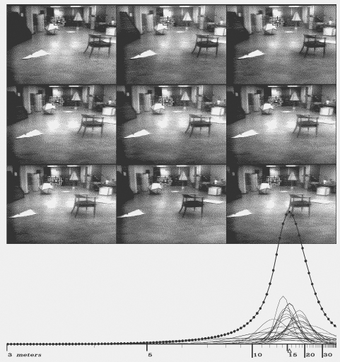
Figure 7.2: Ranging a distant feature

 

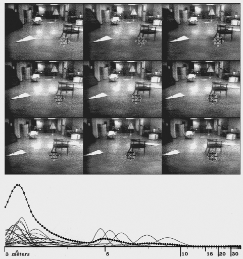
Figure 7.3: Ranging in the presence of a correlation error. Note the mis-match in the last image. Correct feature pairs accumulate probability at the correct distance, while pairs with the incorrect feature dissipate their probability over a spread of distances.

 

The camera slides parallel to the horizontal axis of the (distortion corrected) camera co-ordinate system, so the parallax-induced apparent displacement of features from frame to frame in the 9 pictures is purely in the X direction.

The correlator looks for the points chosen in the central image in each of the eight other pictures. The search is restricted to a narrow horizontal band. This has little effect on the computation time, but it reduces the probability of incorrect matches.

In the case of correct matches, the distance to the feature is inversely proportional to its displacement from one image to another. The uncertainty in such a measurement is the difference in distance a shift one pixel in the image would make. The uncertainty varies inversely with the physical separation of the camera positions where the pictures were taken (the stereo baseline). Long baselines give more accurate distance measurements..

After the correlation step the program knows a feature's position in nine images. It considers each of the 36 ($={9 \choose 2}$) possible image pairings as a stereo baseline, and records the estimated distance to the feature (actually inverse distance) in a histogram. Each measurement adds a little normal curve to the histogram, with mean at the estimated distance, and standard deviation inversely proportional to the baseline, reflecting the uncertainty. The area under the each curve is made proportional to the product of the correlation coefficients of the matches in the two images (in central image this coefficient is taken as unity), reflecting the confidence that the correlations were correct. The area is also scaled by the normalized dot products of X axis and the shift of the features in each of the two baseline images from the central image. That is, a distance measurement is penalized if there is significant motion of the feature in the Y direction.

The distance to the feature is indicated by the largest peak in the resulting histogram, if this peak is above a certain threshold. If below, the feature is forgotten about.

The correlator frequently matches features incorrectly. The distance measurements from incorrect matches in different pictures are usually inconsistent. When the normal curves from 36 pictures pairs are added up, the correct matches agree with each other, and build up a large peak in the histogram, while incorrect matches spread themselves more thinly. Two or three correct correlations out of the eight will usually build a peak sufficient to offset a larger number of errors.

In this way eight applications of a mildly reliable operator interact to make a very reliable distance measurement. Figures 7-1 through 7-3 show typical rangings. The small curves are measurements from individual picture pairs, the beaded curve is the final histogram.

Motion Stereo

The cart navigates exclusively by vision. It deduces its own motion from the apparent 3D shift of the features around it.

After having determined the 3D location of objects at one position, the computer drives the cart about a meter forward.

At the new position it slides the camera and takes nine pictures. The correlator is applied in an attempt to find all the features successfully located at the previous position. Feature descriptions extracted from the central image at the last position are searched for in the central image at the new stopping place.

Slider stereo then determines the distance of the features so found from the cart's new position. The program now knows the 3D position of the features relative to its camera at the old and the new locations. It can figure out its own movement by finding the 3D co-ordinate transform that relates the two.

There can be mis-matches in the correlations between the central images at two positions and, in spite of the eight way redundancy, the slider distance measurements are sometimes in error. Before the cart motion is deduced, the feature positions are checked for consistency. Although it doesn't yet have the co-ordinate transform between the old and new camera systems, the program knows the distance between pairs of positions should be the same in both. It makes a matrix in which element $[i,j]$ is the absolute value of the difference in distances between points $i$ and $j$ in the first and second co-ordinate systems divided by the expected error (based on the one pixel uncertainty of the ranging).

Figure 7.4: The feature list before and after the mutual-distance pruning step. In this diagram the boxes represent features whose three dimensional position is known.

Figure 7.5: Another pruning example, in more difficult circumstances. Sometimes the pruning removed too many points. The cart collided with the cardboard tree to the left later in this run.

Each row of this matrix is summed, giving an indication of how much each point disagrees with the other points. The idea is that while points in error disagree with virtually all points, correct positions agree with all the other correct ones, and disagree only with the bad ones.

The worst point is deleted, and its effect is removed from the remaining points in the row sums. This pruning is repeated until the worst error is within the error expected from the ranging uncertainty.

After the pruning, the program has a number of points, typically 10 to 20, whose position error is small and pretty well known. The program trusts these, and records them in its world model, unless it had already done so at a previous position. The pruned points are forgotten forevermore.

Now comes the co-ordinate transform determining step. We need to find a three dimensional rotation and translation that, if applied to the co-ordinates of the features at the first position, minimizes the sum of the squares of the distances between the transformed first co-ordinates and the raw co-ordinates of the corresponding points at the second position. Actually the quantity that's minimized is the foregoing sum, but with each term divided by the square of the uncertainty in the 3D position of the points involved, as deduced from the one pixel shift rule. This weighting does not make the solution more difficult.

The error expression is expanded. It becomes a function of the rotation and translation, with parameters that are the weighted averages of the $x$, $y$ and $z$ co-ordinates of the features at the two positions, and averages of their various cross-products. These averages need to be determined only once, at the begining of the transform finding process.

To minimize the error expression, its partial derivative with respect to each variable is set to zero. It is relatively easy to simultaneously solve the three linear equations thus resulting from the vector offset, getting the optimal offset values for a general rotation. This gives symbolic expressions (linear combinations of the rotation matrix coefficients) for each of the three vector components. Substituting these values into the error expression makes it a function of the rotation alone. This new, translation determined, error expression is used in all the subsequent steps.

Minimizing the error expression under rotation is surprisingly difficult, mainly because of the non-linear constraints in the 3D rotation matrix. The next six paragraphs outline the struggle. Each step was forced by the inadequacies of the previous one.

The program begins by ignoring the non-linearities. It solves for the general 3D linear transformation, nine elements of a matrix, that minimizes the least square error. The derivatives of the error expression with respect to each of the matrix coefficients are equated to zero, and the nine resulting simultaneous linear equations are solved for the nine coefficients. If the points had undergone an error-free rigid rotation and translation between the two positions, the result would be the desired rotation matrix, and the problem would be solved.

Because there are errors in the determined position of the features, the resulting matrix is usually not simply a rotation, but involves stretching and skewing. The program ortho-normalizes the matrix. If the position errors were sufficiently small, this new matrix would be our answer.

The errors are high enough to warrant adding the rigid rotation constraints in the least squares minimization. The error expression is converted from a linear expression in nine matrix coefficients into an unavoidably non-linear function in three parameters that uniquely characterize a rotation.

This new error expression is differentiated with respect to each of the three rotation parameters, and the resulting expressions are equated to zero, giving us three non-linear equations in three unknowns. A strenuous attempt at an analytic solution of this simultaneous non-linear system failed, so the program contains code to solve the problem iteratively, by Newton's method.

The rotation expressed by the ortho-normalized matrix from the previous step becomes the initial approximation. Newton's method for a multi-variate system involves finding the partial derivative of each expression whose root is sought with respect to each variable. In our case there are three variables and three equations, and consequently nine such derivatives. The nine derivatives, each a closed form expression of the rotation variables, are the coefficients of a 3 by 3 covariance matrix that characterizes the first order changes in the expressions whose roots are sought with the parameters. The next Newton's method approximation is found by multiplying the inverse of this matrix by the value of the root expressions, and subtracting the resulting values (which will be 0 at the root) from the parameter values of the previous approximation.

Four or five iterations usually brings the parameters to within our floating point accuracy of the correct values. Occasionally, when the errors in the determined feature locations are high, the process does not converge. The program detects this by noting the change in the original error expression from iteration to iteration. In case of non-convergence, the program picks a random rotation as a new starting point, and tries again. It is willing to try up to several hundred times. The rotation with the smallest error expression ever encountered during such a search (including the initial approximation) is returned as the answer.

Since the summations over the co-ordinate cross-products are done once and for all at the begining of the transformation determination, each iteration, involving evaluation of about a dozen moderately large expressions and a 3 by 3 matrix inversion, is relatively fast. The whole solving process, even in cases of pathological non-convergence, takes one or two seconds of computer time.

Appendix 7 presents the mathematics of the transform finder in greater detail.

Chapter 8: Path Planning

The cart vision system has an extremely simple minded approach to the world. It models everything it sees as clusters of points. If enough such points are found on each nearby object, this model is adequate for planning a non-colliding path to a destination.

The features in the cart's 3D world model can be thought of as fuzzy ellipsoids, whose dimensions reflect the program's uncertainty of their position. Repeated applications of the interest operator as the cart moves cause virtually all visible objects to be become modelled as clusters of overlapping ellipsoids.

To simplify the problem, the ellipsoids are approximated by spheres. Those spheres sufficiently above the floor and below the cart's maximum height are projected on the floor as circles. The cart itself is modelled as a 3 meter circle. The path finding problem then becomes one of maneuvering the cart's 3 meter circle between the (usually smaller) circles of the potential obstacles to a desired location.

It is convenient (and equivalent) to conceptually shrink the cart to a point, and add its radius to each and every obstacle. An optimum path in this environment will consist of either a straight run between start and finish, or a series of tangential segments between the circles and contacting arcs (imagine loosely laying a string from start to finish between the circles, then pulling it tight).

Superficially, the problem seems to be one of finding the shortest path in a graph of connected vertices. The tangential segments are the edges of the graph, the obstacles, along with the destination and source, are the vertices. There are algorithms (essentially breadth first searches, that repeatedly extend the shortest path to any destination encountered) which, given the graph, can find the desired path in $O(n^2)$ time, where $n$ is the number of vertices. On closer inspection, a few complications arise when we try to apply such an algorithm.

There are four possible paths between each pair of obstacles (Figure 8.1). because each tangent can approach clockwise or counterclockwise. Expanding each obstacle into two distinct vertices, one for clockwise circumnavigations, the other for counterclockwise paths, handles this.

Figure 8.1: The four tangential paths between circular obstacles A and B

Setting up the distance matrix of the graph involves detecting which of the tangential paths are not allowed, because they blocked by other obstacles (such blocked paths are represented by infinite distances). There are $O(n^2)$ tangent paths between obstacle pairs. Determining whether each particular path is blocked involves examining at least a fraction of the other obstacles, a process that takes $O(n)$ time. Thus generating the distance graph, whether explicitly before running the shortest path algorithm, or implicitly within the algorithm itself, takes $O(n^3)$ time. With this consideration, the algorithm is $O(n^3)$.

The obstacles are not dimensionless points. Arriving on one tangent and leaving on another also involves travel on the circular arc between the tangents. Furthermore, paths arriving at an obstacle tangentially from different places do not end up at the same place. Our circular obstacles occupy a finite amount of space. Both these considerations can be handled by noting that the there are only a finite number of tangent points around each obstacle we need consider, and these tangent points are dimensionless.

Each obstacle develops four tangent points because of the existence of every other obstacle. A path problem with $n$ circular obstacles can thus be translated exactly into a shortest path in graph problem with $4n(n-1)$ vertices, each edge in the graph corresponding to a tangent between two obstacles plus the arc leading from one end of the tangent path to the beginning of another one. The solution time thus appears to grow to $O(n^4)$. Fundamentally, this is correct, but significant shortcuts are possible.

Figure 8.2: The shortest path finder's solution to a randomly constructed problem. The route is from the lower left corner to the uper right. The numbered circles are the obstacles, the wiggly line is the solution.

Figure 8.3: Another path finder solution

Figure 8.4: A case where the approximate and exact methods differed. Top diagram is the exact solution, bottom one is the approximate algorithm's guess.

The distance matrix for the tangent points is extremely sparse. In our possible solution space, each tangent point leading from an obstacle connects to only about $2n$ others, out of the $4n(n-1)$ possible. This fact can be used to reduce the amount of work from $O(n^4)$ to about $O(n^3)$. Appendix 8 gives the details.

The algorithm just outlined finds the guaranteed shortest obstacle avoiding path from start to finish. It is rather expensive in time, and especially in space. It requires several two dimensional arrays of size $n$ by $n$. The number of obstacles sometimes grows to be about 100. Because both storage and running time needed conservation, the final version of the cart program used a simplified, and considerably cheaper, approximation to this approach.

The simplified program, also described in greater detail in Appendix 8, does not distinguish between different tangent points arriving at a single obstacle. Instead of a very sparse distance matrix of size $4n(n-1)$ squared, it deals with a dense matrix of dimension $2n$ by $2n$. Many of the arrays that were of size $n^2$ in the full algorithm are only of dimension $n$ in the cheap version. The arc lengths for travel between tangents are added into the computed distances, but sometimes too late to affect the search. If the obstacles were all of zero radius, this simple algorithm would still give an exact solution. As obstacle size grows, so does the probability of non-optimal solutions.

In randomly generated test cases containing about fifty typical obstacles, the approximation finds the best solution about 90% of the time. In the other cases it produces solutions only slightly longer.

A few other considerations are essential in the path planning. The charted routes consist of straight lines connected by tangent arcs, and are thus plausible paths for the cart, which steers like an automobile. This plausibility is not necessarily true of the start of the planned route, which, as presented thus far, does not take the initial heading of the cart into account. The plan could, for instance, include an initial segment going off 90° from the direction in which the cart points, and thus be impossible to execute.

The current code handles this problem by including a pair of “phantom” obstacles along with the real perceived ones. The phantom obstacles have a radius equal to the cart's minimum steering radius, and are placed, in the planning process, on either side of the cart at such a distance that after their radius is augmented by the cart's radius (as happens for all the obstacles), they just touch the cart's centroid, and each other, with their common tangents being parallel to the direction of the cart's heading. They effectively block the area made inaccessible to the cart by its maneuverability limitations.

In the current program the ground plane, necessary to decide which features are obstacles, and which are not, is defined a priori, from the known height of the cart camera above the floor, and the angle of the camera with respect to the horizontal (measured before a run by a protractor/level). Because the program runs so slowly that the longest feasible travel distance is about 20 meters, this is adequate for now. In later, future, versions the cart should dynamically update its ground plane orientation model by observing its own motion as it drives forward. The endpoints of each meter-long lurch define a straight line that is parallel to the local ground. The vector component of the ground plane model in the direction of the lurch can be tilted to match the observed cart motion, while the component perpendicular to that is be left unchanged. After moving in two non-colinear lurches, all ground-plane orientation parameters would be updated. This process would allow the cart to keep its sanity while traversing hilly terrain. Because the motion determination has short term inaccuracies, the tilt model should be updated only fractionally at each move, in the manner of exponential smoothing.

Path Execution

After the path to the destination has been chosen, a portion of it must be implemented as steering and motor commands and transmitted to the cart. The control system is primitive. The drive motor and steering motors may be turned on and off at any time, but there exists no means to accurately determine just how fast or how far they have gone. The current program makes the best of this bad situation by incorporating a model of the cart that mimics, as accurately as possible, the cart's actual behavior. Under good conditions, as accurately as possible means about 20%; the cart is not very repeatable, and is affected by ground slope and texture, battery voltage, and other less obvious externals.

Figure 8.5: An example of the simulator's behavior. The diagram is a plan view of the path executer's world model; the grid cells are one meter on a side. The cart's starting position and final destination and orientation are indicated by arrows. The two large circles, only portions of which are visible, represent the analytic two-arc path. It goes from Start through the tangent of the two circles to Finish. The heavier paths between the two points represent the iterations of the simulator as its parameters were adjusted to compensate for the cart's dynamic response.

The path executing routine begins by excising the first 0.75 meters of the planned path. This distance was chosen as a compromise between average cart velocity, and continuity between picture sets. If the cart moves too far between picture digitizing sessions, the picture will change too much for reliable correlations. This is especially true if the cart turns (steers) as it moves. The image seen by the camera then pans across the field of view. The cart has a wide angle lens that covers 60° horizontally. The 0.75 meters, combined with the turning radius limit (5 meters) of the cart results in a maximum shift in the field of view of 15°, one quarter of the entire image.

This 0.75 meter segment can't be followed precisely, in general, because of dynamic limits in the cart motion. The cart can steer reliably only when it is driving. It takes a finite time for the steering motor to operate. When the drive motors are energized the robot takes a while to accelerate to its terminal velocity, and it coasts for a half meter when the motors are turned off. These complications were too difficult to model in the obstacle path planning.

Instead the program examines the cart's position and orientation at the end of the desired 0.75 meter lurch, relative to the starting position and orientation. The displacement is characterized by three parameters; displacement forward, displacement to the right and change in heading. In closed form the program computes a path that will accomplish this movement in two arcs of equal radius, but different lengths. The resulting trajectory has a general “S” shape. This closed form has three parameters; the radius of the two arcs, the distance along the first arc and the distance along the second, just the right number for a constrained solution of the desired displacement.

Making the arcs of equal radius minimizes the curvature of the planned path, a desirable goal for a vehicle that steers slowly (as well as unreliably). Even with minimized curvature, the two-arc path can only be approximated, since the steering takes a finite amount of time, during which the robot must be rolling.

I was unable to find a closed form expressing the result of simultaneous steering and driving, so the program relys on a simulation. The on and off times for the drive motor necessary to cause the cart to cover the required distance are computed analytically, as are the steering motor on times necessary to set the cart turning with the correct radii. These timings are then fed to the simulator and the final position of the cart is examined. Because the steering was not instantaneous, the simulated path usually turns out to be less curvy than the requested one. The difference between the simulated final position and orientation and the desired one is used to generate a new input for the analytic solver (To clarify; if the simulation says the cart ends up one meter too far to the right, the next iteration will request a position one meter leftward. This process works well when the results of the simulation react nearly linearly to the initial requests). About five iterations of this step are usually sufficient to find an adequate command sequence. This sequence is then transmitted, and the cart moves, more or less as simulated.

Except for the endpoints, the path generated in this way differs, in general, from the one produced by the obstacle avoider algorithm. For 0.75 meter lurches, however, it stays within a few centimeters of it. The cart avoids each obstacle by a safety factor of about a half meter, so such inaccuracies can be tolerated. In any case, the mechanical precision of the cart's response is poor enough, and its seeing sparse enough, to require such a safety margin.

Chapter 9: Evaluation

 

Many years ago I chose the line of research described herein intending to produce a combination of hardware and software by which the cart could visually navigate reliably in most environments. For a number of reasons, the existing system is only a first approximation to that youthful ideal.

One of the most serious limitations is the excruciating slowness of the program. In spite of my best efforts, and many compromises, in the interest of speed, it takes 10 to 15 minutes of real time to acquire and consider the images at each lurch, on a lightly loaded KL-10. This translates to an effective cart velocity of 3 to 5 meters an hour. Interesting obstacle courses (2 or three major obstacles, spaced far enough apart to permit passage within the limits of the cart's size and maneuverability) are at least 15 meters long, so interesting cart runs take from 3 to 5 hours, with little competition from other users, impossibly long under other conditions.

During the last few weeks of the AI lab's residence in the D.C. Power building, when the full fledged obstacle runs described here were executed, such conditions of light load were available on only some nights, between 2 and 6 AM and on some weekend mornings. The cart's video system battery lifetime on a full charge is at most 5 hours, so the limits on field tests, and consequently on the debug/improve loop, were strictly circumscribed.

Although major portions of the program had existed and been debugged for several years, the complete obstacle avoiding system (including fully working hardware, as well as programs) was not ready until two weeks before the lab's scheduled move. The first week was spent quashing unexpected trivial bugs, causing very silly cart behavior under various conditions, in the newest parts of the code, and recalibrating camera and motor response models.

The final week was devoted to serious observation (and filming) of obstacle runs. Three full (about 20 meter) runs were completed, two indoors and one outdoors. Two indoor false starts, aborted by failure of the program to perceive an obstacle, were also recorded. The two long indoor runs were nearly perfect.

In the first, the cart successfully slalomed its way around a chair, a large cardboard icosahedron, and a cardboard tree then, at a distance of about 16 meters, encountered a cluttered wall and backed up several times trying to find a way around it.

The second indoor run involved a more complicated set of obstacles, arranged primarily into two overlapping rows blocking the goal. The cart backed up twice to negotiate the tight turn required to go around the first row, then executed several steer forward / back up moves, lining itself up to go through a gap barely wide enough in the second row. This run had to be terminated, sadly, before the cart had gone through the gap because of declining battery charge and increasing system load.

Figure 9.1: A sample output from the three dimensional drawing program that inspired the construction of the ill fated cardboard trees and rocks

Figure 9.2: Gray scale output from the 3D program. See how seductive the pictures are?

The outdoor run was less successful. It began well; in the first few moves the program correctly perceived a chair directly in front of the camera, and a number of more distant cardboard obstacles and sundry debris. Unfortunately, the program's idea of the cart's own position became increasingly wrong. At almost every lurch, the position solver deduced a cart motion considerably smaller than the actual move. By the time the cart had rounded the foreground chair, its position model was so far off that the distant obstacles were replicated in different positions in the cart's confused world model, because they had been seen early in the run and again later, to the point where the program thought an actually existing distant clear path was blocked. I restarted the program to clear out the world model when the planned path became too silly. At that time the cart was four meters in front of a cardboard icosahedron, and its planned path lead straight through it. The newly re-incarnated program failed to notice the obstacle, and the cart collided with it. I manually moved the icosahedron out of the way, and allowed the run to continue. It did so uneventfully, though there were continued occasional slight errors in the self position deductions. The cart encountered a large cardboard tree towards the end of this journey and detected a portion of it only just in time to squeak by without colliding.

The two short abortive indoor runs involved setups nearly identical to the two-row successful long run described one paragraph ago. The first row, about three meters in front of the cart's starting position contained a chair, a real tree (a small cypress in a planting pot), and a polygonal cardboard tree. The cart saw the chair instantly and the real tree after the second move, but failed to see the cardboard tree ever. Its planned path around the two obstacles it did see put it on a collision course with the unseen one. Placing a chair just ahead of the cardboard tree fixed the problem, and resulted in a successful run. Never, in all my experience, has the code described in this thesis failed to notice a chair in front of the cart.

Flaws Found

These runs suggest that the system suffers from two serious weaknesses. It does not see simple polygonal (bland and featureless) objects reliably, and its visual navigation is fragile under certain conditions. Examination of the program's internal workings suggests some causes and possible solutions.

Bland Interiors

The program sometimes fails to see obstacles lacking sufficient high contrast detail within their outlines. In this regard, the polygonal tree and rock obstacles I whimsically constructed to match diagrams from a 3D drawing program, were a terrible mistake. In none of the test runs did the programs ever fail to see a chair placed in front of the cart, but half the time they did fail to see a pyramidal tree or an icosahedral rock made of clean white cardboard. These contrived obstacles were picked up reliably at a distance of 10 to 15 meters, silhouetted against a relatively unmoving (over slider travel and cart lurches) background, but were only rarely and sparsely seen at closer range, when their outlines were confused by a rapidly shifting background, and their bland interiors provided no purchase for the interest operator or correlator. Even when the artificial obstacles were correctly perceived, it was by virtue of only two to four features. In contrast, the program usually tracked five to ten features on nearby chairs.

It may seem ironic that my program does poorly in the very situations that were the only possible environment for one of its predecessors, SRI's Shakey. Shakey's environment was a large scale “blocks world”, consisting entirely of simple, uniformly colored prismatic solids. Its vision was edge based and monocular, except that it occasionally used a laser range finder to augment its model based 3D reasoning. My area correlation techniques were chosen to work in highly complex and textured “real world” surroundings. That they do poorly in blocks world contexts suggests complementarity. A combination of the two might do better than either alone.

A linking edge follower could probably find the boundary of, say, a pyramidal tree in each of two disparate pictures, even if the background had shifted severely. It could do a stereo matching by noting the topological and geometric similarities between subsets of the edge lists in the two pictures. Note that this process would not be a substitute for the area correlation used in the current program, but an augmentation of it. Edge finding is expensive and not very effective in the highly textured and detailed areas that abound in the real world, and which are area correlation's forte.

Another matching method likely to be useful in some scene areas is region growing, guided by very small scale area correlation.

In the brightly sunlit outdoor run the artificial obstacles had another problem. Their white coloration turned out to be much brighter than any “naturally” occurring extended object. These super bright, glaring, surfaces severely taxed the very limited dynamic range of the cart's vidicon/digitizer combination. When the icosahedron occupied 10% of the camera's field of view, the automatic target voltage circuit in the electronics turned down the gain to a point where the background behind the icosahedron appeared nearly solid black.

Confused Maps

The second major problem exposed by the runs is glitches in the cart's self-position model. This model is updated after a lurch by finding the 3D translation and rotation that best relates the 3d position of the set of tracked features before and after the lurch. In spite of the extensive pruning that precedes this step, (and partly because of it, as is discussed later) small errors in the measured feature positions sometimes cause the solver to converge to the wrong transform, giving a position error well beyond the expected uncertainty. Features placed into the world model before and after such a glitch will not be in the correct relative positions. Often an object seen before is seen again after, now displaced, with the combination of old and new positions combining to block a path that is in actuality open.

This problem showed up mainly in the outdoor run. I've also observed it indoors in past, in simple mapping runs, before the entire obstacle avoider was assembled. There appear to be two major causes for it, and a wide range of supporting factors.

Poor seeing, resulting in too few correct correlations between the pictures before and after a lurch, is one culprit. The highly redundant nine eyed stereo ranging is very reliable, and causes few problems, but the non-redundant correlation necessary to relate the position of features before and after a lurch, is error prone. Features which have been located in 3D from one picture ninetuplet are sought in the next set by applying the correlator between the central images of the two sets. The points so found are then ranged using nine eyed stereo in the new picture set. The cart's motion is deduced by finding the apparent 3D movement of the features from one picture set to the next.

Before this 3D co-ordinate transformation is computed, the matched points are pruned by considering their mutual three dimensional distances in the two co-ordinate systems. Accurate to the known position uncertainty of each feature, these distances should be the same in the two systems. Points that disagree in this measure with the majority of other points are rejected.

If too few points are correctly matched, because the seeing was poor, or the scene was intrinsically too bland, the pruning process can go awry. This happened several times in the outdoor run.

The outdoor scene was very taxing for the cart's vidicon. It consisted of large regions (mainly my cardboard constructions) glaring in direct sunlight, and other important regions in deep shadow. The color of the rest of the scene was in a relatively narrow central gray range. It proved impossible to simultaneously not saturate the glaring or the shadowed areas, and to get good contrast in the middle gray band, within the six bit (64 gray level) resolution of my digitized pictures. To make matters even more interesting, the program ran so slowly that the shadows moved significantly (up to a half meter) between lurches. Their high contrast boundaries were favorite points for tracking, enhancing the program's confusion.

Simple Fixes

Though elaborate (and thus far untried in our context) methods such as edge matching may greatly improve the quality of automatic vision in future, subsequent experiments with the program revealed some modest incremental improvements that would have solved most of the problems in the test runs.

The issue of unseen cardboard obstacles turns out to be partly one of over-conservatism on the program's part. In all cases where the cart collided with an obstacle it had correctly ranged a few features on the obstacle in the prior nine-eyed scan. The problem was that the much more fragile correlation between vehicle forward moves failed, and the points were rejected in the mutual distance test. Overall the nine-eyed stereo produced very few errors. If the path planning stage had used the pre-pruning features (still without incorporating them permanently into the world model) the runs would have proceeded much more smoothly. All of the most vexing false negatives, in which the program failed to spot a real obstacle, would have been eliminated. There would have been a very few false positives, in which non-existent ghost obstacles would have been perceived. One or two of these might have caused an unnecessary swerve or backup. But such ghosts would not pass the pruning stage, and the run would have proceeded normally after the initial, non-catastrophic, glitch.

The self-position confusion problem is related, and in retrospect may be considered a trivial bug. When the path planner computes a route for the cart, another subroutine takes a portion of this plan and implements it as a sequence of commands to be transmitted to the cart's steering and drive motors. During this process it runs a simulation that models the cart acceleration, rate of turning and so on, and which provides a prediction of the cart's position after the move. With the current hardware the accuracy of this prediction is not great, but it nevertheless provides much a priori information about the cart's new position. This information is used, appropriately weighted, in the least-squares co-ordinate system solver that deduces the cart's movement from the apparent motion in 3D of tracked features. It is not used, however, in the mutual distance pruning step that preceeds this solving. When the majority of features have been correctly tracked, failure to use this information does not hurt the pruning. But when the seeing is poor, it can make the difference between choosing a spuriously agreeing set of mis-tracked features and the small correctly matched set.

Incorporating the prediction into the pruning, by means of a heavily weighted point that the program treats like another tracked feature, removes almost all the positioning glitches when the program is fed the pictures from the outdoor run.

I have not attempted any live cart runs with these program changes because the cramped conditions in our new on-campus quarters make cart operations nearly impossible.

Chapter 10: Spinoffs

Graphics

The display hardware in the early days of the AI lab was strictly vector oriented; six vector terminals from Information International Inc., and a Calcomp plotter. When I arrived at Stanford the lab had just acquired a new raster based display system from Data Disc Corp. The display packages in existence at the time, of which there were several, had all started life in the vector environment, and were all oriented around vector list display descriptions. Some of the packages had been extended by addition of routines that scanned such a vector list and drew the appropriate lines in a Data Disc raster.

In my opinion, this approach had two drawbacks if raster displaying was to supplant vector drawing. The vector list is compact for simple pictures, but can grow arbitrarily large for complex pictures with many lines. A pure raster representation, on the other hand, needs a fixed amount of storage for a given raster size, independent of the complexity of the image in the array. I often saw programs using the old display packages bomb when the storage allocated for their display lists was exceeded. A second objection to vector list representations is that they had no elegant representation for some of the capabilities of raster devices not shared by vector displays, notably large filled in areas.

These thoughts prompted me to write a raster oriented display package for the Data Disc monitors that included such primitives as ellipse and polygon filling (including convex and star polygons), darkening and inversion as well as lighting of filled areas, in addition to the traditional linear commands. This package has developed a large following, and has been translated into several languages (the original package was written to run in a SAIL environment. Portions of it have been modified to run in raw assembly code, and under Lisp 1.6 \ref{W2} and Maclisp \ref{B1} \ref{L1}). It is outlined in Appendix 10.

Figure 10.1: A silly picture produced from a GOD file. The little program which wrote the file may be found in Appendix 10

The Data Disc package was built around a rather peculiar and inflexible raster format (for instance, the raster lines are four-way interleaved) made necessary by the nature of the Data Disc hardware. When our XGP arrived there was no easy way to extend it to handle buffers for both the Data Disc and the much higher resolution XGP, though I did add a small routine which produced a coarse XGP page by expanding each Data Disc raster pixel.

Thus the arrival of the XGP created the need for a new package which could generate high resolution XGP images from calls similar to the ones used with Data Disc. I fashioned one by modifying the innermost parts of a copy of the older routines.

New raster devices were appearing,and a single system able to handle all of them became clearly desirable. The general byte raster format used in the vision package described later in this chapter was a good medium for implementing such generality, and I once again made a modified version of the Data Disc package which this time drew into arbitrary rectangular subwindows of arbitrarily sized bit rasters. I added a few new features, such as the ability to deposit characters from XGP font files and halftone pictures into the drawing. Only partially implemented at this writing is a package which draws into byte rasters, using gray scale to produce images with reduced edge jagginess.

With both hard and soft copy graphic output devices available it became desirable to write programs which drew the same picture into buffers of different resolutions destined for different devices. Since the buffers were sometimes very large, it was reasonable to put them in separate core images. Thus evolved a message based version of the graphics routines in which the graphics main program does none of the actual drawing itself, but creates graphic “slaves” which run as separate jobs, and to which it sends messages such as “draw a line from [1.5,2.3] to [5.2,0.1].” A large number of such graphic servers can exist at any one time, and they can be individually activated and deactivated at any time. Whenever the controlling program executes a graphics primitive, all the servers currently active do the appropriate drawing. The messages sent to graphics servers can also be written into files (which can be created, destroyed, activated and deactivated just as if they were servers). Such files, which I call GOD files (for Graphics On Displays, Documents and other Devices), can be saved and used to generate drawings off-line, by manually feeding them to any of the available graphics servers. GOD files can also be used as subroutines in later drawing programs, and in more powerful ways, as suggested in the next paragraph.

A version of these routines is at the core of XGPSYN and XGPSYG, programs which can display pages from .XGP multifonted documentation files readably as gray scale images on standard TV monitors, as well as being able to list them on the XGP, after composing them as full bit rasters. XGPSYG, additionally, can insert diagrams and halftone representations of gray scale pictures into the documents being printed, in response to escape sequences occurring in the documents, pointing to GOD graphic files, hand eye format picture files or Leland Smith's music manuscript plot files (!).

Figure 10.2: Another GOD file example. This diagram was produced with the help of a circuit drawing extension to the main package

The obstacle avoider program used the message graphics system to document its internal state, generating in the process some of the diagrams seen in this thesis. The text in the thesis was formatted with Don Knuth's TEX typesetting system \ref{K1}, and printed with diagrams using XGPSYG.

Vision Software

The Hand-Eye project had collected a moderately large package of utility subroutines for acquiring and analysing pictures when I began my vision work. Unfortunately it was far from complete, even in its basics, and was built around a “global” picture representation (global variables held picture size and location parameters) which made dealing with several pictures at the same time nearly impossible, especially if they were of different sizes. This was a great handicap to me since I worked nearly from the start with hierarchies of reduced pictures, and with excerpted windows. The format also made certain primitive operations, such as individual byte accessing, unnecessarily difficult because it carried insufficient precomputed data.

In my opinion there was little worth salvaging, so I began writing my own vision primitives from scratch, starting with a data representation that included with each picture constants such as the number of words in a scanline, as well as a table of byte pointer skeletons for accessing each column. It features high speed in the utility operations, and in such fancier things as correlation and filtering. It has a clever digitizing subroutine that compensates for some of the limitations of our hardware. This package has grown over the years and is now considerably more extensive than the Hand Eye library, and has largely supplanted it in other Stanford vision projects \ref{B2}.

The obstacle avoider uses an extension of the basic package which permits convenient handling of sequences of successively reduced pictures, and of chains of windows excerpted from such sequences.

PIX is a program that uses the vision subroutines to provide desk calculator type services for pictures to a user. It can digitize pictures from various sources, transform and combine them in many ways, transfer them to and from disk, display or print them on various output devices. Among its more exotic applications has been the generation of font definitions for our printer from camera input. XGPSYN and XGPSYG also make use of the vision package. The 3D shaded graphics in this thesis were produced with a program that uses the partially implemented gray scale GOD file server, which also calls on the vision package.

Further details may be found in Appendix 10.