R语言空间数据分析学习笔记5——栅格数据处理
geo&R
1 十进制转二进制
library(R.utils)
#原始二进制
paste(intToBin(41190))
[1] "1010000011100110"
#保存为32位二进制
(paste(rev(as.integer(intToBits(41190))),collapse = ""))
[1] "00000000000000001010000011100110"
#获取16位二进制
substr(paste(rev(as.integer(intToBits(41190))),collapse = ""),17,32)
[1] "1010000011100110"
# paste(intToBin(1025))
# (paste(rev(as.integer(intToBits(1024))),collapse = ""))
# substr(paste(rev(as.integer(intToBits(1024))),collapse = ""),22,22)
for (i in seq_along(MODIS$StateQA)){
MODIS$QA2bin[i] <- substr(paste(rev(as.integer(intToBits(MODIS$StateQA[i]))),collapse = ""),22,22)
}
2 按条件求和求平均
2.1 按月份求月均气温和月累计降水
library(readxl)
mydf = read_excel(path = "C:\\Users\\Administrator\\Desktop\\data1124\\climate\\Climate.xls")
View(mydf)
class(mydf)
class(mydf$Date)
mydf$month <- format(mydf$Date, '%Y-%m')
mydf$month <- format(mydf$Date, '%Y-%m')
mydf
month1 <- data.frame(a = tapply(mydf$平均气温, mydf$month, mean),
a = tapply(mydf$最高气温, mydf$month, mean),
a = tapply(mydf$最低气温, mydf$month, mean),
b = tapply(mydf$日累计降水, mydf$month, sum))
write.csv(month1,file = "C:\\Users\\Administrator\\Desktop\\data1124\\climate\\month.csv")
3 R语言读取矢量和栅格
参考:知乎大v:HopeR
感谢!
pacman:Package Management Tool
sf:simple feature of R
raster:Geographic Data Analysics and Modeling
GADM:The Global Administrative area database
crs:coordinate reference system
IDW(inverse distance weighted interpolation)
library(pacman)
p_load(sf, raster, tidyverse)
# 查看有哪些图层
st_layers(
"H:/shp/gadm36_KEN_gpkg/gadm36_KEN.gpkg"
)
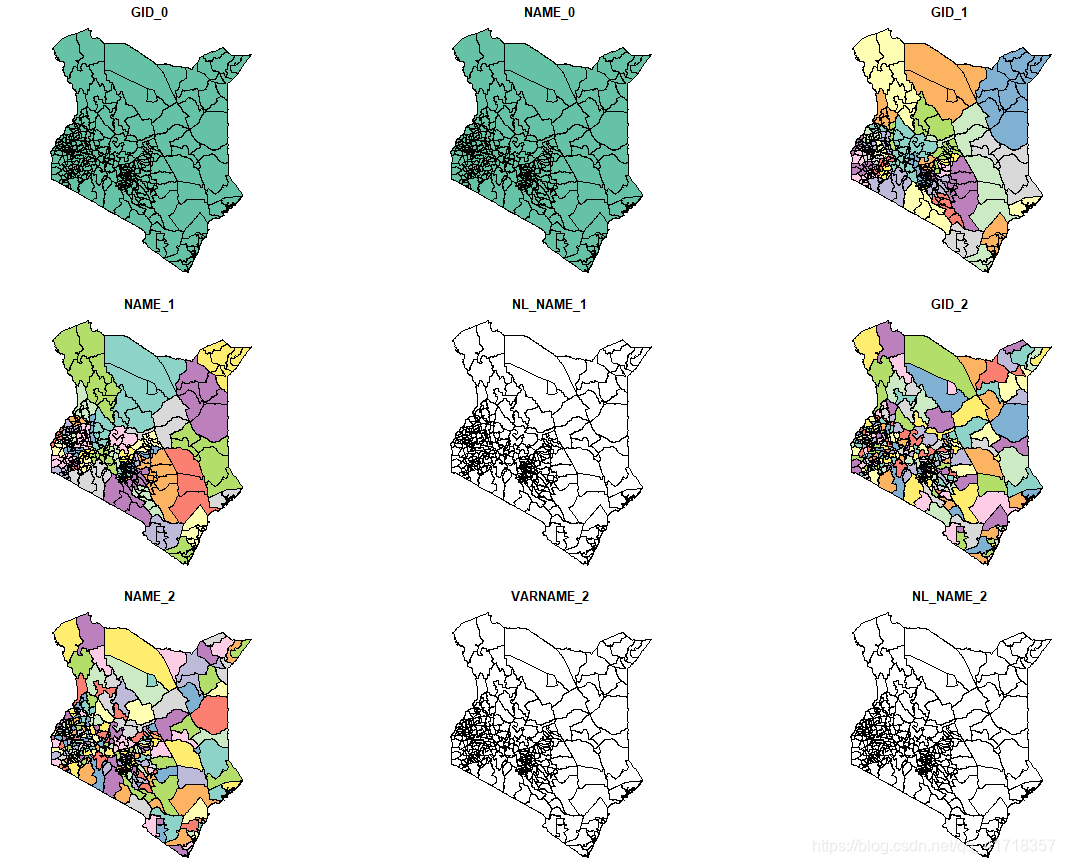
Kenoutline <- st_read("H:/shp/gadm36_KEN_gpkg/gadm36_KEN.gpkg",
layer='gadm36_KEN_2')
#打印这个数据
print(Kenoutline)
#查看其坐标系
st_crs(Kenoutline)
# Coordinate Reference System:
# User input: WGS 84
# wkt:
# GEOGCRS["WGS 84",
# DATUM["World Geodetic System 1984",
# ELLIPSOID["WGS 84",6378137,298.257223563,
# LENGTHUNIT["metre",1]]],
# PRIMEM["Greenwich",0,
# ANGLEUNIT["degree",0.0174532925199433]],
# CS[ellipsoidal,2],
# AXIS["geodetic latitude (Lat)",north,
# ORDER[1],
# ANGLEUNIT["degree",0.0174532925199433]],
# AXIS["geodetic longitude (Lon)",east,
# ORDER[2],
# ANGLEUNIT["degree",0.0174532925199433]],
# USAGE[
# SCOPE["unknown"],
# AREA["World"],
# BBOX[-90,-180,90,180]],
# ID["EPSG",4326]]
plot(Kenoutline)
读取栅格数据
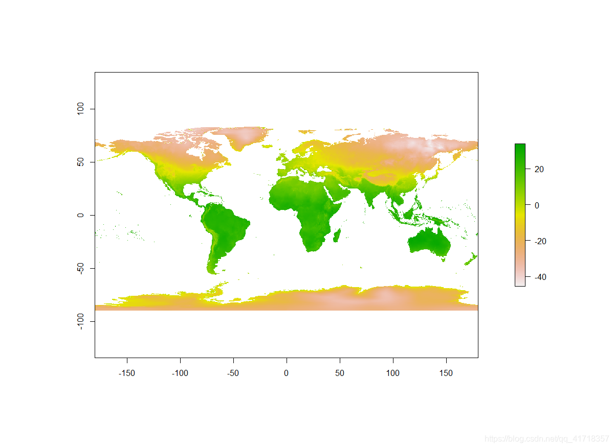
tempreture<-raster("H:/shp/wc2.1_10m_tavg/wc2.1_10m_tavg_01.tif")
tempreture
# class : RasterLayer
# dimensions : 1080, 2160, 2332800 (nrow, ncol, ncell)
# resolution : 0.1666667, 0.1666667 (x, y)
# extent : -180, 180, -90, 90 (xmin, xmax, ymin, ymax)
# crs : +proj=longlat +datum=WGS84 +no_defs
# source : H:/shp/wc2.1_10m_tavg/wc2.1_10m_tavg_01.tif
# names : wc2.1_10m_tavg_01
# values : -45.884, 34.0095 (min, max)
st_crs(tempreture)
# Coordinate Reference System:
# User input: +proj=longlat +datum=WGS84 +no_defs
# wkt:
# GEOGCRS["unknown",
# DATUM["World Geodetic System 1984",
# ELLIPSOID["WGS 84",6378137,298.257223563,
# LENGTHUNIT["metre",1]],
# ID["EPSG",6326]],
# PRIMEM["Greenwich",0,
# ANGLEUNIT["degree",0.0174532925199433],
# ID["EPSG",8901]],
# CS[ellipsoidal,2],
# AXIS["longitude",east,
# ORDER[1],
# ANGLEUNIT["degree",0.0174532925199433,
# ID["EPSG",9122]]],
# AXIS["latitude",north,
# ORDER[2],
# ANGLEUNIT["degree",0.0174532925199433,
# ID["EPSG",9122]]]]
plot(tempreture)
改变栅格投影坐标系
newproj<-"+proj=moll +lon_0=0 +x_0=0 +y_0=0 +ellps=WGS84 +datum=WGS84 +units=m +no_defs"
tempreture1<-tempreture%>%projectRaster(crs = newproj)
plot(tempreture1)
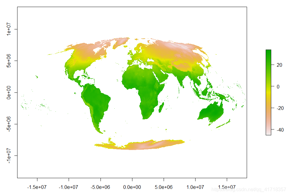
%>%来自dplyr包的管道函数,其作用是将前一步的结果直接传参给下一步的函数,从而省略了中间的赋值步骤,可以大量减少内存中的对象,节省内存。
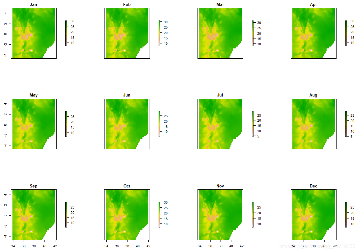
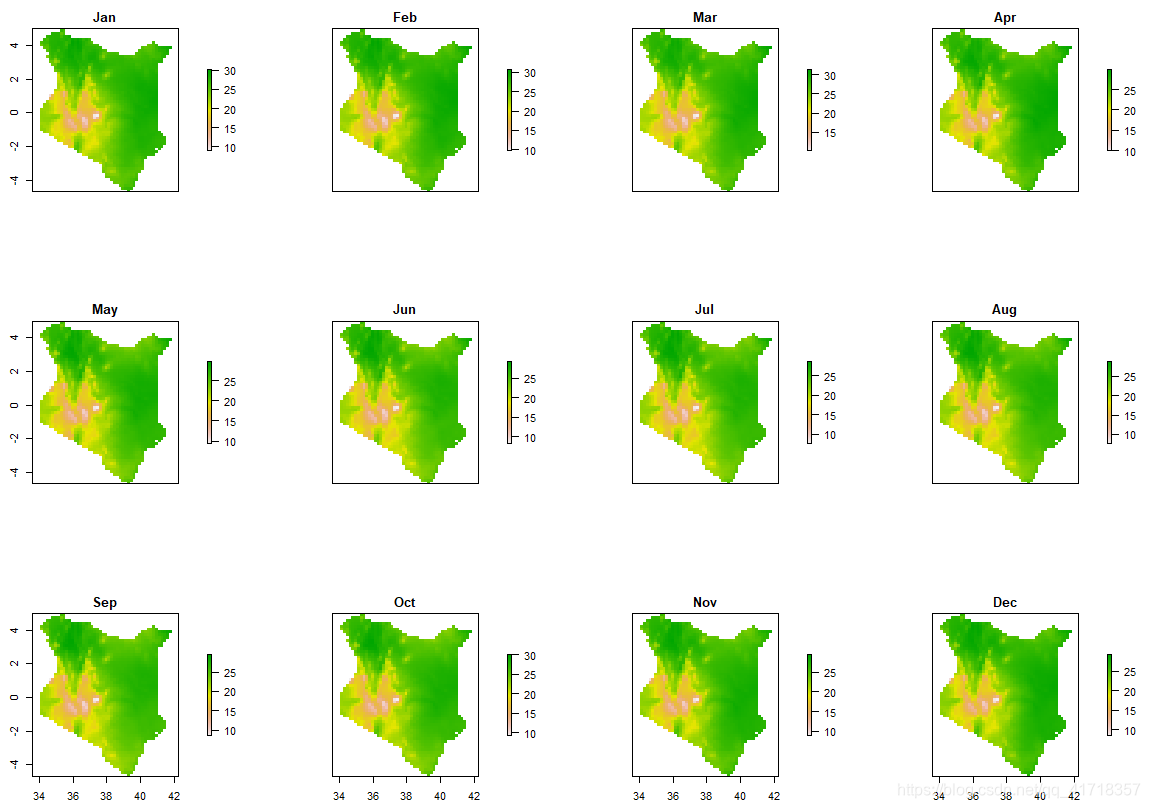
一次读入所有栅格数据
#一次读入所有栅格数据
dir("G:/shp/wc2.1_10m_tavg",full.names = TRUE)%>%
stack()->worldclimate
worldclimate
# class : RasterStack
# dimensions : 1080, 2160, 2332800, 12 (nrow, ncol, ncell, nlayers)
# resolution : 0.1666667, 0.1666667 (x, y)
# extent : -180, 180, -90, 90 (xmin, xmax, ymin, ymax)
# crs : +proj=longlat +datum=WGS84 +no_defs
# names : wc2.1_10m_tavg_01, wc2.1_10m_tavg_02, wc2.1_10m_tavg_03, wc2.1_10m_tavg_04, wc2.1_10m_tavg_05, wc2.1_10m_tavg_06, wc2.1_10m_tavg_07, wc2.1_10m_tavg_08, wc2.1_10m_tavg_09, wc2.1_10m_tavg_10, wc2.1_10m_tavg_11, wc2.1_10m_tavg_12
# min values : -45.88400, -44.80000, -57.92575, -64.19250, -64.81150, -64.35825, -68.46075, -66.52250, -64.56325, -55.90000, -43.43475, -45.32700
# max values : 34.00950, 32.82425, 32.90950, 34.19375, 36.25325, 38.35550, 39.54950, 38.43275, 35.79000, 32.65125, 32.78800, 32.82525
month<-c("Jan","Feb","Mar","Apr","May","Jun",
"Jul","Aug","Sep","Oct","Nov","Dec")
names(worldclimate)<-month
worldclimate
worldclimate$[[1]]
worldclimate$Jan
# class : RasterStack
# dimensions : 1080, 2160, 2332800, 12 (nrow, ncol, ncell, nlayers)
# resolution : 0.1666667, 0.1666667 (x, y)
# extent : -180, 180, -90, 90 (xmin, xmax, ymin, ymax)
# crs : +proj=longlat +datum=WGS84 +no_defs
# names : Jan, Feb, Mar, Apr, May, Jun, Jul, Aug, Sep, Oct, Nov, Dec
# min values : -45.88400, -44.80000, -57.92575, -64.19250, -64.81150, -64.35825, -68.46075, -66.52250, -64.56325, -55.90000, -43.43475, -45.32700
# max values : 34.00950, 32.82425, 32.90950, 34.19375, 36.25325, 38.35550, 39.54950, 38.43275, 35.79000, 32.65125, 32.78800, 32.82525
#提取特定城市的温度数据
Kenoutline$NAME_1
site<-c("Mombasa", "Nakuru", "Meru","Marsabit","Kakuma")
lon<-c(39.655,36.8172,37.64561,38.01902,34.85441)
lat<-c(-4.0412,-1.28962,0.05186,2.33916,3.71634)
#put all of this information into one list
samples<-data.frame(site,lon,lat,row.names = "site")
samples
# Exctrct the data from the Rasterstack for all point
KenCityTemp<-raster::extract(worldclimate,samples)
class(KenCityTemp)
KenCityTemp
# Jan Feb Mar Apr May Jun Jul Aug Sep Oct Nov Dec
# [1,] 27.19083 27.56361 28.08833 27.31250 25.74750 24.70750 23.78306 23.92917 24.62333 25.64444 26.59528 27.02778
# [2,] 19.37425 19.99025 20.23750 19.65600 18.58350 17.18000 16.34900 16.65275 17.83250 19.15825 18.91300 18.67950
# [3,] 17.17025 17.95600 18.43675 17.91850 17.32725 16.31475 15.75400 16.03425 17.35950 18.02175 17.15275 16.67075
# [4,] 24.05100 24.76150 24.79825 23.70475 23.18525 22.18050 21.42425 21.66375 22.63575 23.05825 22.76675 23.13600
# [5,] 27.90425 28.59675 28.63800 27.48875 27.30100 26.96225 26.41325 26.43175 27.30975 27.54900 27.32775 27.19650
KenCityTemp2<- KenCityTemp %>%
as_tibble()%>%
add_column(Site=site,.before="Jan")
KenCityTemp2
# Site Jan Feb Mar Apr May Jun Jul Aug Sep Oct Nov Dec
# <chr> <dbl> <dbl> <dbl> <dbl> <dbl> <dbl> <dbl> <dbl> <dbl> <dbl> <dbl> <dbl>
# 1 Mombasa 27.2 27.6 28.1 27.3 25.7 24.7 23.8 23.9 24.6 25.6 26.6 27.0
# 2 Nakuru 19.4 20.0 20.2 19.7 18.6 17.2 16.3 16.7 17.8 19.2 18.9 18.7
# 3 Meru 17.2 18.0 18.4 17.9 17.3 16.3 15.8 16.0 17.4 18.0 17.2 16.7
# 4 Marsabit 24.1 24.8 24.8 23.7 23.2 22.2 21.4 21.7 22.6 23.1 22.8 23.1
# 5 Kakuma 27.9 28.6 28.6 27.5 27.3 27.0 26.4 26.4 27.3 27.5 27.3 27.2
从世界气温图中裁剪出肯尼亚的部分,使用crop函数
Kentemp<-Kenoutline %>%
#now crop our temp data to the extent
crop(worldclimate,.)
Kentemp
# class : RasterBrick
# dimensions : 58, 49, 2842, 12 (nrow, ncol, ncell, nlayers)
# resolution : 0.1666667, 0.1666667 (x, y)
# extent : 33.83333, 42, -4.666667, 5 (xmin, xmax, ymin, ymax)
# crs : +proj=longlat +datum=WGS84 +no_defs
# source : memory
# names : Jan, Feb, Mar, Apr, May, Jun, Jul, Aug, Sep, Oct, Nov, Dec
# min values : 7.00550, 7.59825, 7.86850, 7.01375, 6.01350, 5.03775, 4.30050, 4.78400, 5.54800, 6.64600, 6.82000, 6.88075
# max values : 30.18350, 30.95450, 31.74950, 30.16625, 29.74000, 29.21300, 28.52475, 28.69950, 29.58900, 30.09900, 29.56600, 29.33750
#plot the output
plot(Kentemp)
裁剪出真正属于肯尼亚的部分
exactKen<-Kentemp %>%
mask(Kenoutline,na.rm=TRUE)
plot(exactKen)
或者可以这样(一步到位):
Kentemp<-Kenoutline %>%
#now crop our temp data to the extent
crop(worldclimate,.) %>%
mask(.,Kenoutline,na.rm = TRUE)
Kentemp
#plot the output
plot(Kentemp)
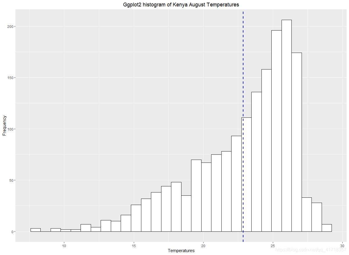
对肯尼亚八月份的数据做一个温度直方图
#可以尝试对8月份的数据做一个温度分布直方图
Kentempdf<-Kentemp %>%
as.data.frame()
#set up the basic histogram
gghist<-ggplot(Kentempdf,
aes(x=Aug))+
geom_histogram(color="black",
fill="white")+
labs(title="Ggplot2 histogram of Kenya August Temperatures",
x="Temperatures",
y="Frequency")
#add a vertical line to the histogram showing mean temperature
gghist + geom_vline(aes(xintercept=mean(Aug,
na.rm=TRUE)),
color="blue",
linetype="dashed",
size=1)+
theme(plot.title = element_text(hjust = 0.5))
空间插值之前,先合并气温的时空分布数据
#最后,我们会演示一下空间插值的过程。首先,我们来合并气温的时空分布数据:
samplestemp<-KenCityTemp%>%
cbind(samples)
samplestemp
# Jan Feb Mar Apr May Jun Jul Aug Sep Oct Nov Dec
# Mombasa 27.19083 27.56361 28.08833 27.31250 25.74750 24.70750 23.78306 23.92917 24.62333 25.64444 26.59528 27.02778
# Nakuru 19.37425 19.99025 20.23750 19.65600 18.58350 17.18000 16.34900 16.65275 17.83250 19.15825 18.91300 18.67950
# Meru 17.17025 17.95600 18.43675 17.91850 17.32725 16.31475 15.75400 16.03425 17.35950 18.02175 17.15275 16.67075
# Marsabit 24.05100 24.76150 24.79825 23.70475 23.18525 22.18050 21.42425 21.66375 22.63575 23.05825 22.76675 23.13600
# Kakuma 27.90425 28.59675 28.63800 27.48875 27.30100 26.96225 26.41325 26.43175 27.30975 27.54900 27.32775 27.19650
# lon lat
# Mombasa 39.65500 -4.04120
# Nakuru 36.81720 -1.28962
# Meru 37.64561 0.05186
# Marsabit 38.01902 2.33916
# Kakuma 34.85441 3.71634
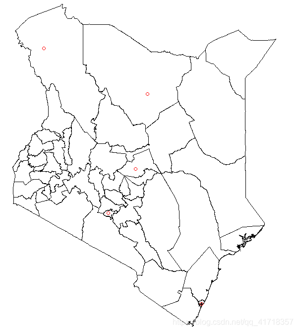
然后把它转化为空间信息数据框,这里需要声明经纬所在列,以及坐标系定义为4326(WGS 84)
#然后把它转化为空间信息数据框,这里需要声明经纬所在列,以及坐标系定义为4326
samplestemp<-samplestemp%>%
st_as_sf(.,coords=c("lon","lat"),
crs=4326,
agr="constant")#
samplestemp
plot(Kenoutline$geometry)
plot(st_geometry(samplestemp),add=TRUE)
插值之前让我们先统一坐标系,然后转化为sp对象
samplestemp
# Simple feature collection with 5 features and 12 fields
# Attribute-geometry relationship: 12 constant, 0 aggregate, 0 identity
# geometry type: POINT
# dimension: XY
# bbox: xmin: 34.85441 ymin: -4.0412 xmax: 39.655 ymax: 3.71634
# geographic CRS: WGS 84
# Jan Feb Mar Apr May Jun Jul Aug Sep Oct Nov Dec
# Mombasa 27.19083 27.56361 28.08833 27.31250 25.74750 24.70750 23.78306 23.92917 24.62333 25.64444 26.59528 27.02778
# Nakuru 19.37425 19.99025 20.23750 19.65600 18.58350 17.18000 16.34900 16.65275 17.83250 19.15825 18.91300 18.67950
# Meru 17.17025 17.95600 18.43675 17.91850 17.32725 16.31475 15.75400 16.03425 17.35950 18.02175 17.15275 16.67075
# Marsabit 24.05100 24.76150 24.79825 23.70475 23.18525 22.18050 21.42425 21.66375 22.63575 23.05825 22.76675 23.13600
# Kakuma 27.90425 28.59675 28.63800 27.48875 27.30100 26.96225 26.41325 26.43175 27.30975 27.54900 27.32775 27.19650
# geometry
# Mombasa POINT (39.655 -4.0412)
# Nakuru POINT (36.8172 -1.28962)
# Meru POINT (37.64561 0.05186)
# Marsabit POINT (38.01902 2.33916)
# Kakuma POINT (34.85441 3.71634)
samplestemp<-samplestemp%>%
st_transform(21097)
samplestemp
Kenoutline<-Kenoutline%>%
st_transform(21097)
samplestempsp<-samplestemp%>%
as(.,'Spatial')
Kenoutlinesp<-Kenoutline%>%
as(.,'Spatial')
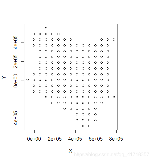
#现在意味着我们要用手头若干个城市的数值,来对澳大利亚的气温空间分布进行插值,
#我们需要创建一个要插值的空间范围
emptygrd<-as.data.frame(spsample(Kenoutlinesp,n=1000,type = "regular",cellsize=60000))
names(emptygrd)<-c("X", "Y")
plot(emptygrd)
coordinates(emptygrd)<-c("X", "Y")
gridded(emptygrd)<-TRUE #create SpatialPixel object
fullgrid(emptygrd)<-TRUE #create SpatialGrid object
#add the projection to the grid
proj4string(emptygrd)<-proj4string(samplestempsp)
#然后进行插值:
p_load(gstat)
#Interpolate the grid cells using a power value of 2
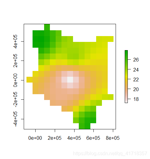
interpolate<-gstat::idw(Jan~1, samplestempsp, newdata=emptygrd, idp=2.0)
#这里使用IDM算法来插值,只使用1月份的数据,idp参数越大,则随着距离的增大,
#数值减少越大。如果idp为0,那么随着距离加大,依然不会有任何数值衰减。
#convert output to raster object
ras<-raster(interpolate)%>%
mask(.,Kenoutline)
plot(ras)
参考资料:
https://andrewmaclachlan.github.io/CASA0005repo/rasters-descriptive-statistics-and-interpolation.html
https://zhuanlan.zhihu.com/p/280968987
欢迎关注公众号Geosuper

腾讯云面向开发者汇聚海量精品云计算使用和开发经验,营造开放的云计算技术生态圈。
更多推荐


 13
13 0
0- 0


 已为社区贡献2条内容

所有评论(0)