机械臂动力学——动力学建模

一、动力学方程基本动力学模型τ　＝　D(q)q¨+C(q,q˙)+G(q)\tau　＝　D(q)\ddot{q}+C(q,\dot{q})+G(q)τ　＝　D(q)q¨+C(q,q˙)+G(q)τ\tauτ为关节力矩，D(q)D(q)D(q)为机械臂的n×nn \times nn×n质量矩阵，C(q,q˙)C(q,\dot{q})C(q,q˙)为n×1n \times 1n×1离心...

文章共68,574字 · 阅读需要大约229分钟

一键AI生成摘要，助你高效阅读

问答

white_Learner

36459人浏览 · 2019-10-17 17:51:15

white_Learner · 2019-10-17 17:51:15 发布

一、动力学基础概念

基本动力学模型
$\tau ＝ D(q)\ddot{q}+C(q,\dot{q})+G(q)$

$\tau$ 为关节力矩， $D (q)$ 为机械臂的 $\times n$ 质量矩阵， $C(q,\dot{q})$ 为 $\times 1$ 离心力和科氏力矢量， $G (q)$ 为 $\times 1$ 的重力矢量

建模方法

牛顿-欧拉法
拉格朗日法

连杆质量，连杆质心位置矢量，连杆质心惯性矩阵（通过动力学参数识别获得）

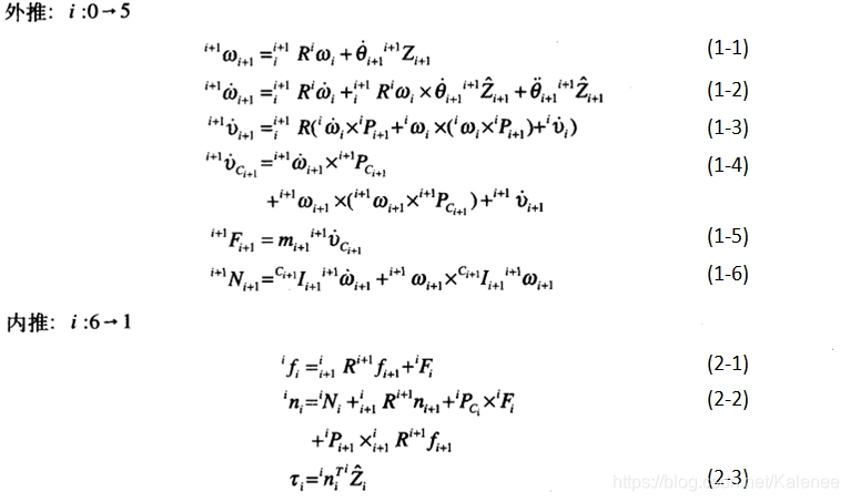
二、牛顿-欧拉法

运动外推：向外迭代计算连杆的角速度、角加速度和线加速度
力外推：计算作用在连杆质心上的惯性力和力矩
力矩内推：向内迭代计算关节力矩

2.1 运动向外迭代

2.1.1 刚体线速度和角速度

线速度

坐标系{A}为固定，坐标系{B}固连在刚体上。

$^{A}V_Q$ 为Q点在坐标系{A}的速度； $^{B}V_Q$ 为Q点在坐标系{B}的速度； $^{A}_{B}R$ 为坐标系{B}相对于坐标系{A}的变换矩阵； $^{A}V_{BORG}$ 为位置矢量的导数。
$^{A}V_Q = ^{A}V_{BORG} + ^{A}_{B}R\ ^{B}V_Q$

该方程适用于两个坐标系相对方位保持不变。

角速度

坐标系原点重合，线速度为零。

$^{B}Q$ 为矢量，确定了坐标系{B}中一个固定点的位置； $^{A}\Omega_B$ 为 $^{B}Q$ 相对于坐标系{A}的角速度； $^{A}V_Q$ 为Q点在坐标系{A}的速度； $^{B}V_{Q}$ 为Q点在坐标系{B}的速度； $^{A}_{B}R$ 为坐标系{B}相对于坐标系{A}的变换矩阵。
$^{A}V_Q =^{A}_{B}R \ ^{B}V_{Q} + ^{A}\Omega_B \times ^{A}_{B}R\ ^{B}Q$

线速度+角速度

从坐标系{A}观测坐标系{B}中固定速度矢量的普遍公式
$^{A}V_Q =^{A}V_{BORG} + ^{A}_{B}R \ ^{B}V_{Q} + ^{A}\Omega_B \times ^{A}_{B}R\ ^{B} Q$

2.1.2 连杆速度

连杆i+1的速度为连杆i的速度加上附加到关节i+1上的速度分量。

注意：线速度相对于一点，角速度相对于一个物体，因此，"连杆的速度“指连杆坐标原点的线速度和连杆的角速度

角速度

连杆i+1的角速度等于连杆i的角速度加上一个由于关节i+1上的角速度引起的分量。
$^{i}w_{i+1} = ^{i}w_{i}+\ _{i+1}^{i}R \dot{\theta}_{i+1}\ ^{i+1}\hat{Z}_{i+1}\\ \dot{\theta}_{i+1}\ ^{i+1}\hat{Z}_{i+1} = ^{i+1}\begin{bmatrix} 0\\0\\\dot{\theta}_{i+1} \end{bmatrix}$

两边同时左乘 $_{i}^{i+1}R$ 可获得连杆i+1的角速度相对于坐标系{i+1}表达式：
$^{i+1}w_{i+1} = _{i}^{i+1}R\ ^{i}w_{i}+ \dot{\theta}_{i+1}\ ^{i+1}\hat{Z}_{i+1} \tag{1-1}$

对 $\theta$ 求导
$^{i+1}\dot{w}_{i+1} = _{i}^{i+1}R\ ^{i}\dot{w}_{i}+ _{i}^{i+1}R\ ^{i}w_{i}\times \dot{\theta}_{i+1}\ ^{i+1}\hat{Z}_{i+1} +\ddot{\theta}_{i+1}\ ^{i+1}\hat{Z}_{i+1} \tag{1-2}$

线速度

坐标系{i+1}原点的线速度等于坐标系{i}原点的线速度加上一个由于连杆i的角速度引起的新的分量。（ $P_{i+1}$ 为位置矢量）

从坐标原点指向质点所在位置的矢量称为位置矢量，简称位矢
直角坐标系： $\hat{i} + y \hat{j} +z \hat{k}$

$^{i}v_{i+1} = ^{i}v_{i}+\ ^{i}w_i \times ^{i}P_{i+1}$

两边同时左乘 $_{i}^{i+1}R$ ：
$^{i+1}v_{i+1} = _{i}^{i+1}R(^{i}v_{i}+\ ^{i}w_i \times ^{i}P_{i+1})$

对位置矢量 $P$ 求导为
$^{i+1}\dot{v}_{i+1} = _{i}^{i+1}R(^{i}\dot{w}_i \times ^{i}P_{i+1}+ ^{i}w_i \times (^{i}w_i \times ^{i}P_{i+1})+^{i}\dot{v}_{i}) \tag{1-3,1-4}$

2.2 力向外迭代

2.2.1 牛顿方程（Newton）

在这里插入图片描述
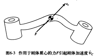
用于描述刚体的平动。

质点的牛顿方程
$\ddot{r} = F$
$m$ 为质点质量， $r$ 为矢径， $\ddot{r}$ 为加速度， $F$ 为质点的合力。

平动刚体的牛顿方程

刚体平动为刚体上每一点速度一致。
$\ddot{r_p} = F$
$\ddot{r_p}$ 为刚体上任一点加速度。

一般运动刚体的牛顿方程

刚体平动为刚体上各点速度不相同。
$\ddot{r_c} = F \tag{1-5}$

$\ddot{r_c}$ 为刚体质心的加速度。

2.2.2 欧拉方程（Euler方程）

在这里插入图片描述
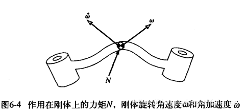
绕定点转动刚体的Euler方程
$M_o = I_o \dot{w} + w \times I_o w \tag{1-6}$

$w$ 为刚体固连坐标系的角速度， $I_o$ 为常值矩阵，表示刚体在与刚体固连坐标系中对O点的惯性张量矩。

2.3 力和力矩向内迭代

在这里插入图片描述
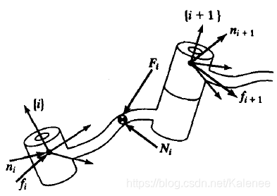
上图为典型连杆在无重力状态下受力图，根据该图建立力平衡方程和力矩平衡方程。

力平衡方程

$^{i}F_i = ^{i}f_i - ^{i}_{i+1}R^{i+1}f_{i+1}$

$f_i$ 为连杆i-1作用在连杆i上的力

力矩平衡方程

$^{i}N_i = ^{i}n_i - ^{i}n_{i+1} + (-^{i}P_{C_i}) \times ^{i}f_i - (^{i}P_{i+1}-^{i}P_{C_i}) \times ^{i}f_{i+1}$

$n_i$ 为连杆i-1作用在连杆i上的力矩

$^{i}n_{i+1} =^{i}_{i+1}R\ ^{i+1}n_{i+1}\\ ^{i}F_i = ^{i}f_i - ^{i}_{i+1}R^{i+1}f_{i+1} =^{i}F_i = ^{i}f_i - ^{i}f_{i+1}$

根据力平衡方程和附加旋转矩阵可化简该公式

$\begin{aligned} ^{i}N_i &= ^{i}n_i -^{i}_{i+1}R\ ^{i+1}n_{i+1} +(-^{i}P_{C_i}) \times ^{i}f_i - (-^{i}P_{C_i}) \times ^{i}f_{i+1} -^{i}P_{i+1} \times ^{i}f_{i+1}\\ &= ^{i}n_i -^{i}_{i+1}R\ ^{i+1}n_{i+1} -^{i}P_{C_i} \times ^{i}F_i - ^{i}P_{i+1} \times ^{i}_{i+1}R\ ^{i+1}f_{i+1} \end{aligned}$

迭代方程

按照连杆序号高到低排序获得迭代关系为
$^{i}f_i = ^{i}_{i+1}R^{i+1}f_{i+1} + ^{i}F_i \tag{2-1}$

$^{i}n_i = ^{i}N_i + ^{i}_{i+1}R\ ^{i+1}n_{i+1}+ ^{i}P_{C_i} \times ^{i}F_i + ^{i}P_{i+1} \times ^{i}_{i+1}R\ ^{i+1}f_{i+1} \tag{2-2}$

2.4 建立动力学方程

在这里插入图片描述

2.5 两连杆动力学方程

在这里插入图片描述
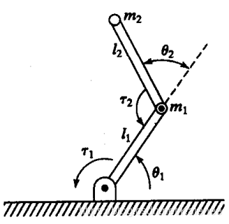
假设连杆质量集中在连杆末端，质量分别为 $m_1$ 和 $m_2$ 。

连杆质心位置矢量

$^{1}P_{c_1} = l_1 \hat{x_1} = \begin{bmatrix}l_1\\0\\0\end{bmatrix}\\^{2}P_{c_2} = l_2 \hat{x_2}= \begin{bmatrix}l_2\\0\\0\end{bmatrix}$

因质量集中，因此连杆质心惯性张量为零矩阵
$^{C_1}I_{1} = 0 \\ ^{C_2}I_{2} = 0$

末端执行器上无作用力

$f_3 =0\\ n_3 =0$

机器人基座为固定

$w_0 =\begin{bmatrix} 0\\0\\0 \end{bmatrix}\\ \dot{w_0} =\begin{bmatrix} 0\\0\\0 \end{bmatrix}$

包括重力因素（在牛顿－欧拉法下，只需要底座包含重力因素，其余连杆可以不考虑重力的影响）

$^{0}\dot{v_0} = g \hat{Y_0} = \begin{bmatrix} 0\\g\\0 \end{bmatrix}$

连杆坐标系之间相对转动
$_{i+1}^{i}R = \begin{bmatrix} c_{i+1} & -s_{i+1} &0 \\ s_{i+1} & c_{i+1} & 0\\ 0 & 0 & 1 \end{bmatrix} ,\\ _{i}^{i+1}R = \begin{bmatrix} c_{i+1} & s_{i+1} &0 \\ -s_{i+1} & c_{i+1} & 0\\ 0 & 0 & 1 \end{bmatrix}$

向外迭代（ $\rightarrow 1$ ）

连杆1
连杆2

向内迭代（ $\rightarrow 1$ ）
连杆2
连杆1

力矩（取 $^{i}n_{i}$ 中的 $\hat{Z}$ 方向分量，平行与关节的方向）

状态空间方程
$\tau ＝ M(\Theta )\ddot{\Theta }+C(\Theta ,\dot{\Theta })+G(\Theta)\\\tau =\begin{bmatrix}\tau _1\\\tau _2\end{bmatrix}\\$
$\Theta$ 为关节角度矩阵
质量矩阵 $M(\Theta )$

速度项 $V(\Theta,\dot{\Theta} )$ 包含与关节速度相关项

重力项 $G(\Theta )$ 包含了与重力加速度g有关项

Matlab建模

% 动力学建模
syms l1 l2 m1 m2 g;
syms q1 q2 dq1 dq2 ddq1 ddq2;

%% 参数初始化
R{1}=[cos(q1) -sin(q1) 0;sin(q1) cos(q1) 0;0 0 1];
R{2}=[cos(q2) -sin(q2) 0;sin(q2) cos(q2) 0;0 0 1];
R{3}=[1 0 0;0 1 0;0 0 1];
% 坐标系原点位移，用P{1}表示坐标系1与坐标系0原点位置关系，用P{2}表示坐标系2与坐标系1原点位置关系。
P = cell(1,3);
P{1}=[0;0;0];P{2}=[l1;0;0];P{3}=[l2;0;0];
% 每个连杆质心的位置矢量
Pc = cell(1,3);
Pc{1}=[0;0;0];Pc{2}=[l1;0;0];Pc{3}=[l2;0;0];
% 连杆质量
m = cell(1,3);
m{2}=m1;
m{3}=m2;
% 惯性张量
I = cell(1,3);
I{2}=[0;0;0];
I{3}=[0;0;0];

% 连杆间角速度和角加速度
w = cell(1,3);dw = cell(1,3);
w{1}=[0;0;0];dw{1}=[0;0;0];% 机器人底座不旋转
% 连杆坐标原点和质心加速度
dv = cell(1,3);dvc = cell(1,3);
dv{1}=[0;g;0];% 重力因素

% 关节速度和加速度
dq = cell(1,3); ddq = cell(1,3); 
dq{2}=[0;0;dq1];dq{3}=[0;0;dq2];
ddq{2}=[0;0;ddq1];ddq{3}=[0;0;ddq2];

% 末端执行器没有力
f = cell(1,4);n = cell(1,4);
f{4}=[0;0;0];
n{4}=[0;0;0];

%% 建立运动学方程
% 外推
for i=1:2 %matlab下标从1开始
w{i+1}=R{i}.'*w{i}+dq{i+1};
dw{i+1}=R{i}.'*dw{i}+cross(R{i}.'*w{i},dq{i+1})+ddq{i+1};

dv{i+1}=R{i}.'*(cross(dw{i},P{i})+cross(w{i},cross(w{i},P{i}))+dv{i});
dvc{i+1}=cross(dw{i+1},Pc{i+1})+cross(w{i+1},cross(w{i+1},Pc{i+1}))+dv{i+1};

F{i+1}=m{i+1}*dvc{i+1};
N{i+1}=[0;0;0];%假设质量集中，每个连杆惯性张量为0
end

% 内推
for i=3:-1:2
    f{i}=R{i}*f{i+1}+F{i};
    n{i}=N{i}+R{i}*n{i+1}+cross(Pc{i},F{i})+cross(P{i},R{i}*f{i+1});
end

% 力矩
tau = cell(1,2);
tau{1} = n{2}(3);
tau{2} = n{3}(3);
celldisp(tau)

三、拉格朗日法

拉格朗日法为基于能量的动力学方法。

3.1 动能

第i根连杆的动能 $k_i$ 为连杆质心线速度产生动能和连杆角速度产生动能之和
$k_i = \frac{1}{2} v^{T}_{C_i} m_i v_{C_i} + \frac{1}{2} \ ^{i}w_{i}^{T} \ ^{C_i}I_{i} \ ^{i}w_i$

整个机械臂动能为各个连杆动能之和
$\sum_{i+1}^{n} k_i$

$v_c$ 和 $^{i}w_i$ 为 $\Theta$ （关节位置）和 $\dot{\Theta}$ （关节速度）的函数，因此机械臂动能可描述为关节位置和速度的标量函数， $M(\Theta)$ 为机械臂 $\times n$ 的质量矩阵
$k(\Theta,\dot{\Theta}) = \frac{1}{2} \dot{\Theta}^T M(\Theta) \dot{\Theta}$

3.2 势能

第i根连杆的势能 $u_i$ 为
$u_i = - m_i \ ^{0}g^{T} \ ^{0}P_{C_i}+u_{refi}$

$^{0}g$ 为 $\times 1$ 重力矢量， $^{0}P_{C_i}$ 为第i根连杆质心矢量 $\times 1$ ， $u_{refi}$ 是使 $u_i$ 的最小值为零的常数。

$u_{refi}$ 的引入用于表示连杆的势能的参考点，但实际上在动力学方程中，仅计算势能相对于 $\Theta$ 的偏导数 $\frac{\partial u}{\partial \Theta}$ ，因此该常数值可为任意值，即势能可相对于任意一个参考零点。

3.3 构建动力学方程

拉格朗日函数定义为系统的动能减去势能
$\mathcal L(\Theta,\dot{\Theta})=k(\Theta,\dot{\Theta})-u(\Theta)$

操作臂运动方程为
$\frac{d}{dt} \frac{\partial \mathcal L}{\partial \dot{\Theta}}- \frac{\partial \mathcal L}{\partial \Theta}=\tau$

$\tau$ 为 $\times 1$ 力矩矢量，运动方程代入拉格朗日函数为
$\frac{d}{dt} \frac{\partial k}{\partial \dot{\Theta}}- \frac{\partial k}{\partial \Theta}+\frac{\partial u}{\partial \Theta}=\tau$

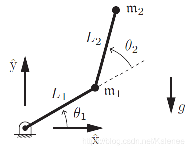
3.4 两连杆动力学方程

2R机械臂在处在xy平面内，重力沿-y方向。

两连杆动力学方程
连杆质心线速度

连杆1

$\left[\begin{matrix} x_1\\ y_1 \end{matrix}\right]= \left[\begin{matrix} L_1 \cos\theta_1\\ L_1 \sin\theta_1 \end{matrix}\right]\\ \left[\begin{matrix} \dot x_1\\ \dot y_1 \end{matrix}\right]= \left[\begin{matrix} -L_1 \sin\theta_1\\ L_1 \cos\theta_1 \end{matrix}\right]\dot \theta_1$

连杆2

$\left[\begin{matrix} x_2\\ y_2 \end{matrix}\right]= \left[\begin{matrix} L_1 \cos\theta_1+L_2 \cos(\theta_1+\theta_2)\\ y_1 \sin\theta_1+L_2 \sin(\theta_1+\theta_2) \end{matrix}\right]\\ \left[\begin{matrix} \dot x_2\\ \dot y_2 \end{matrix}\right]= \left[\begin{matrix} -L_1 \sin \theta_1-L_2 \sin(\theta_1+\theta_2)& -L_2 \sin(\theta_1+\theta_2)\\ L_1 \cos \theta_1+L_2 \cos(\theta_1+\theta_2) & L_2 \cos(\theta_1+\theta_2) \end{matrix}\right] \left[\begin{matrix} \dot\theta_1\\ \dot\theta_2 \end{matrix}\right]$

连杆角速度

因质量集中，连杆质心惯性张量为零矩阵
$^{C_1}I_{1} = 0 \\ ^{C_2}I_{2} = 0$
因此连杆角速度产生动能为0，即
$k_i = \frac{1}{2} v^{T}_{C_i} m_i v_{C_i}$
连杆动能

$\begin{aligned} \mathcal K_1 &=\frac{1}{2}m_1(\dot x_1^2+\dot y_1^2)=\frac{1}{2}m_1L_1^2\dot\theta_1^2\\ \mathcal K_2 &=\frac{1}{2}m_2(\dot x_2^2+\dot y_2^2)\\ &=\frac{1}{2}m_2((L_1^2+2L_1L_2 \cos\theta_2+L_2^2)\dot\theta_1+2(L_2^2+L_1L_2 \cos\theta_2)\dot\theta_1\dot\theta_2+L_2^2\dot\theta_2^2) \end{aligned}$

连杆势能
$\begin{aligned} u_1&=m_1gy_1=m_1gL_1sin\theta_1\\ u_2&=m_2gy_2=m_2g(L_1sin\theta_1+L_2sin(\theta_1+\theta_2)) \end{aligned}$

拉格朗日方程
$\begin{aligned} \mathcal L =& (\mathcal K_1 + \mathcal K_2) - (u_1 +u_2)\\ =& (\frac{1}{2}m_1L_1^2\dot\theta_1^2 + \frac{1}{2}m_2((L_1^2+2L_1L_2 \cos\theta_2+L_2^2)\dot\theta_1+2(L_2^2+L_1L_2 \cos\theta_2)\dot\theta_1\dot\theta_2+L_2^2\dot\theta_2^2)) \\& -(m_1gL_1sin\theta_1+m_2g(L_1sin\theta_1+L_2sin(\theta_1+\theta_2))) \end{aligned}$

使用运动方程求力矩
$\tau_i=\frac{d}{dt}\frac{\partial \mathcal L}{\partial \dot\theta_i}-\frac{\partial \mathcal L}{\theta_i}, i=1,2$

$\begin{aligned} \tau_1 =& (m_1L_1^2+m_2(L_1^2+2L_1L_2 \cos\theta_2+L_2^2))\ddot\theta_1+\\ & m_2(L_1L_2 \cos\theta_2+L_2^2)\ddot\theta_2-m_2L_1L_2 \sin\theta_2(2\dot\theta_1\dot\theta_2+\dot\theta_2^2)+\\ & (m_1+m_2)L_1g \cos\theta_1+m_2gL_2 \cos(\theta_1+\theta_2)\\ \tau_2 = & m_2(L_1L_2 \cos\theta_2+L_2^2)\ddot\theta_1 + m_2L_2^2 \ddot\theta_2 + m_2 L_1 L_2 \dot \theta_1^2 \sin \theta_2 \\ & +m_2gL_2 \cos(\theta_1+\theta_2) \end{aligned}$

状态空间方程
$\begin{aligned} M(\theta)&=\left [ \begin{matrix} m_1L_1^2+m_2(L_1^2+2L_1L_2 \cos\theta_2+L_2^2) &m_2(L_1L_2 \cos\theta_2+L_2^2)\\ m_2(L_1L_2 \cos\theta_2+L_2^2) &m_2L_2^2\\ \end{matrix}\right]\\ c(\theta,\dot\theta)&=\left [ \begin{matrix} -m_2(L_1L_2 \sin\theta_2(2\dot\theta_1\dot\theta_2 +\dot\theta_2^2)\\ m_2L_1L_2\dot\theta_1^2 \sin\theta_2\\ \end{matrix}\right]\\ g(\theta)&=\left [ \begin{matrix} (m_1+m_2)L_1g \cos\theta_1+m_2 g L_2 \cos(\theta_1+\theta_2)\\ m_2 g L_2 \cos(\theta_1+\theta_2)\\ \end{matrix}\right] \end{aligned}$

matlab建模

% 质量集中，无惯性矩阵，连杆长度与质心位置重合
syms m1 m2 l1 l2 g 
syms q1 q2 q1d q2d q1dd q2dd 
syms x1(t) x1d x1dd x2(t) x2d x2dd

x1d=diff(x1,t); x2d=diff(x2,t);
x1dd=diff(x1,t,t); x2dd=diff(x2,t,t);

%质量矩阵
M1=diag([m1,m1]);
M2=diag([m2,m2]);

% 速度
V1=[[l1*cos(x1(t)) 0];[l1*sin(x1(t)) 0]]*[x1d;x2d];
V2=[[-l1*sin(x1(t))-l2*sin(x1(t)+x2(t)) -l2*sin(x1(t)+x2(t))];
    [l1*cos(x1(t))+l2*cos(x1(t)+x2(t)) l2*cos(x1(t)+x2(t))]]*[x1d;x2d];

% 动能
K1=simplify((1/2)*V1.'*M1*V1);
K2=simplify((1/2)*V2.'*M2*V2);
K =K1+K2;

% 势能
u1=m1*g*l1*sin(q1);
u2=m2*g*(l1*sin(q1)+l2*sin(q1+q2));
u =u1+u2;

% 拉格朗日方程
L=K-u;
L=subs(L,{x1,x2,x1d,x2d,x1dd,x2dd},{q1,q2,q1d,q2d,q1dd,q2dd});

% 利用运动方程计算力矩方程
dLdqd=[diff(L,q1d); diff(L,q2d)];
dLdqd =subs(dLdqd, {q1,q2,q1d,q2d,q1dd,q2dd}, {x1,x2,x1d,x2d,x1dd,x2dd});
ddLdqddt=diff(dLdqd,t);
ddLdqddt= subs(ddLdqddt,{x1,x2,x1d,x2d,x1dd,x2dd},{q1,q2,q1d,q2d,q1dd,q2dd});
dLdq=[diff(L,q1); diff(L,q2)];

% 输出结果
syms f
f=simplify(ddLdqddt-dLdq)

四、算法对比

在这里插入图片描述
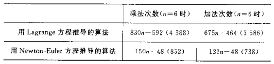
通过牛顿欧拉方程导出的逆动力算法较拉格朗日方程推导计算量要少，但实际上两者差异在于表示连杆角速度的方式不一致，牛顿欧拉方程采用三维矢量，拉格朗日方程采用 $\times 3$ 旋转矩阵导数，因此多余因素造成计算量增大，若在计算动能时采用三维角速度矢量描述，则拉格朗日方程可推导处与牛顿欧拉方程相同的形式的逆动力方程。